REFFERENCES:

WIKIPEDIA, MATH WORKS.COM, TUTORIALS POINT.COM
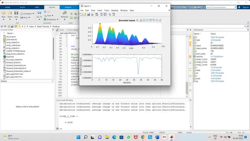
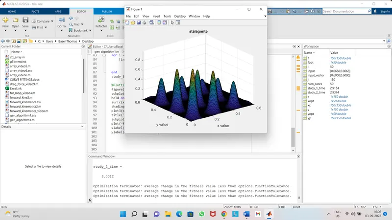
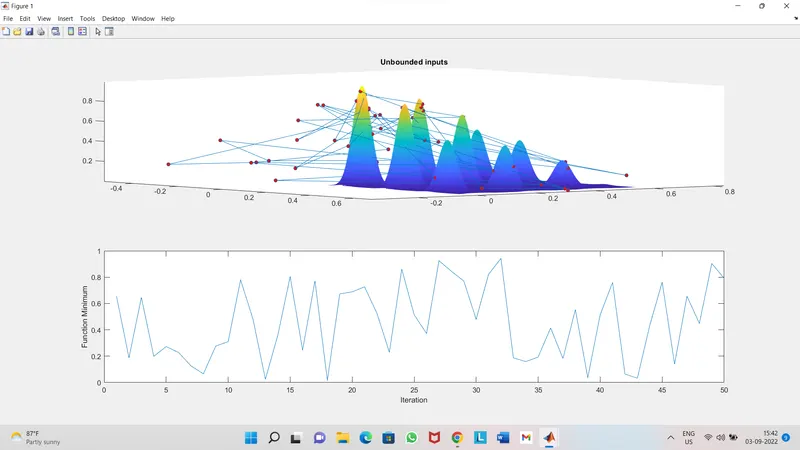
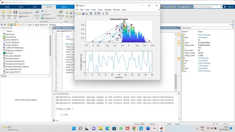
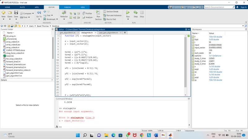
ERRORS;

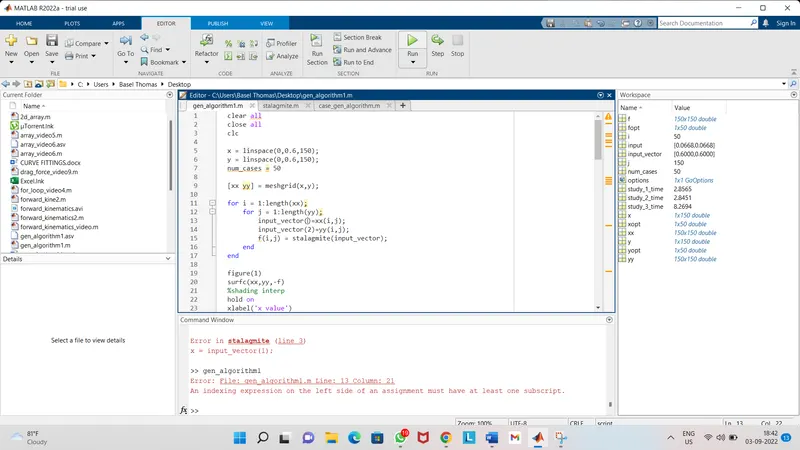
ERROR 1 - Not giving enough input arguement
ERROR 2 - NOt giving the value for input vector

CORRECTIONS;

CORRECTION 1 - Giving proper input arguement mentuoned in the code
CORRECTION 2 - Giving the right value for the input vector
Based on the research, answer for following questions are;

Stopping criteria-
When there has been no improvement in the population for X iterations.

When we reach an absolute number of generations.
When the objective function value has reached a certain pre-defined value.


Syntax for ga-  ga(@stalagmite,2,[ ],[ ],[ ],[ ],[0;0],[1;1],[ ],[ ],options)
ga(fun,nvars,A,b,Aeq,beq,lb,ub,nonlcon,options)

ga -  To find the minimum of function using Genetic Algorithm
fun -  finds a local minimum to function
nvars - number of variables.
A -  Linear Inequality Constraints,specified as a real matrix
b -  Linear Inequality Constraints,specified as a real vector
Aeq - Linear equality Constraints,specified as a real matrix
beq - Linear equality Constraints,specified as a real matrix
lb -  Lower Bound
ub-  Upper Bound
nonlcon - Nonlinear Constraints, specified as function handle
options- Optimization options, specified as the output
EXPLANATION

clear all
close all
clc         - for clearing the memory

x,y variables (input variables) doesnt define the ga & doesnt know its actual value as well. 150 defines the division or limit points in between 0 & 0.6 (population).
x = linspace(0,0.6,150); - creating varable x by using linspace array matrix command
y = linspace(0,0.6,150); - creating varable y by using linspace array matrix command
num_cases = 50 - means im going to run the program for 50 times.

[xx yy] = meshgrid(x,y); - Meshgrid used for the convertion of 1d into 2d array

for i = 1:length(xx); - for loop is used for the calculation of reccuring values obtained for each running operation. i stores the values of the x variables
    for j = 1:length(yy); - j stores the values of the y variables
        input_vector(1)=xx(i,j); - input vector 1(row array vector) is created for saving the each value of x
        input_vector(2)=yy(i,j); - input vector 2(row array vector) is created for saving the each value of y

        f(i,j) = stalagmite(input_vector); - function f(i,j) stores the stalagmite function values inorder to calculate the maxima.
    end - for ending the for loop of j
end - for the the for of i

figure(1) - used for plotting different plots on same figure window
surfc(xx,yy,-f) - for visualising the output for the inputs(xx,yy,-f). -f is because of plotting the fig in opposite direction as that of +f.
%shading interp
hold on - for holding the plot without overwritting
xlabel('x value') - for labeling x axis
ylabel('y value') - for labeling y axis
title('stalagmite') - for putting title for the fig as stalagmite.
num_cases = 50; - for running the program for 50 times

% Case 1| Unbounded Statistics

tic - for the calculation of time taken for the evaluation

for i = 1:num_cases -  for loop is used for finding the values for each reccuring operation
    [input, fopt(i)] = ga(@stalagmite,2); - GA  syntax for the unbounded GA study for
which the lower & upper bounds are not defined. input, fopt(i) stores the values for the genetic algorithm  of our stalagmite function of 2 variables.
    xopt(i) = input(1) xopt(i) stores the input 1 values
    yopt(i) = input(2); - yopt(i) stores the input 2 values
end - for ending the for loop
study_1_time = toc - study 1 times shows the time taken for the execution

%Plotting the Graph
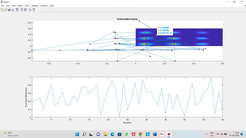
figure(1) - used for plotting different plots on same figure window
subplot(2,1,1) - subplot is used for plotting mutiple figures having 2 rows 1 colomn and show as 1st fig in the plot
hold on - for holding the plot without overwritting

surfc(x,y,-f) - for visualising the output for the inputs(xx,yy,-f). -f is because of plotting the fig in opposite direction as that of +f.
shading interp - for getting a smooth plot with grade lines
plot3(xopt,yopt,-fopt,'marker','o','markersize',5,'markerfacecolor','r') - for plotting the fig with xopt, yopt, -fopt, with a mark of o with a size of 5mm having red color.
title('Unbounded inputs') - for putting title for the fig as unbounded inputs
subplot(2,1,2) subplot is used for plotting mutiple figures having 2 rows
, 1 colomn and second fig in the plot
xlabel('Iteration') -for labeling x axis  as iteration
ylabel('Function Minimum') for labeling x axis  as function minimum

%Case 2 | Bounded Statstics (with lower and upper boundaries)


tic - for the calculation of time taken for the evaluation

for i = 1:num_cases - for loop is used for finding the values for each reccuring operation
    [input, fopt(i)] = ga(@stalagmite,2,[],[],[],[],[0;0],[1;1]); - GA  syntax for the bounded GA study for which the lower & upper bounds are defined as 0 & 1 respectivily, also the square brackets shows the theres no constraints or conditions involved. input, fopt(i) stores the values for the genetic algorithm  of our stalagmite function of 2 variables.
        xopt(i) = input(1); - xopt(i) stores the input 1 values
    yopt(i) = input(2); - yopt(i) stores the input 2 values
end - for ending the for loop-

study_2_time = toc - study 2 times shows the time taken for the execution

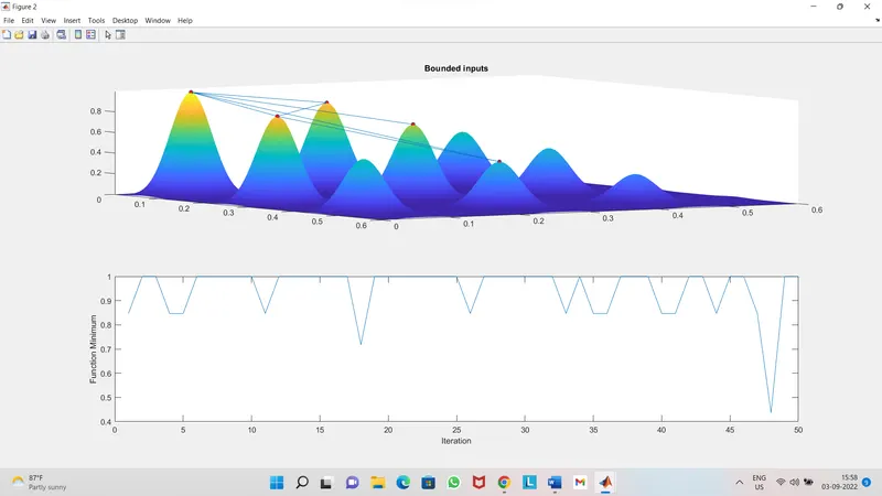
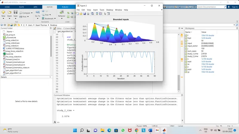
figure(2) - used for plotting different plots on same figure window
subplot(2,1,1) - subplot is used for plotting mutiple figures having 2 rows 1 colomn and show as 1st fig in the plot
hold on - for holding the plot without overwritting

surfc(x,y,-f) - for visualising the output for the inputs(xx,yy,-f). -f is because of plotting the fig in opposite direction as that of +f.
shading interp - for getting a smooth plot with grade lines
plot3(xopt,yopt,-fopt,'marker','o','markersize',5,'markerfacecolor','r') - for plotting the fig with xopt, yopt, -fopt, with a mark of o with a size of 5mm having red color.
title('Bounded inputs') - for putting title for the fig as bounded inputs
subplot(2,1,2) subplot is used for plotting mutiple figures having 2 rows
, 1 colomn and second fig in the plot
xlabel('Iteration') -for labeling x axis  as iteration
ylabel('Function Minimum') for labeling y axis  as function minimum


%Study-3 | Bounded GA study with population size -
In addition with specifying bounds, I am also increasing initial population size.
If population size is too small, we cannot find the global maxima, but
we can find only local maxmia, which happens in study2.
Following the same procedure as in study-2, and increase the population
size to 240 and applying the constraint ‘optimoptions’ and save its values
in variable ‘options’ to allow the ga to predict the optimum solution from 240 population size.
options = optimoptions('ga');
options = optimoptions(options,'PopulationSize',240);

tic  for the calculation of time taken for the evaluation
-
for i = 1:num_cases
    [input, fopt(i)] = ga(@stalagmite,2,[],[],[],[],[0;0],[1;1],[],[],options); - here we have mentioned lower and upper bound as 0and 1 resp. but in addition to that the option describes the increse in the initial population (250) - which inturns helps to find the global maxima instead of local maxima.
        xopt(i) = input(1); - xopt(i) stores the input 1 values
        yopt(i) = input(2); - yopt(i) stores the input 2 values

end for ending the for loop
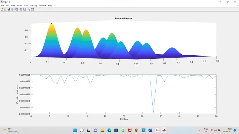
study_3_time = toc for showing the time taken for the execution

% plotting figure
figure(3) - used for plotting different plots on same figure window
subplot(2,1,1) - subplot is used for plotting mutiple figures having 2 rows 1 colomn and show the 1st fig in the plot
hold on - for holding the plot without overwritting

surfc(x,y,-f) - for visualising the output for the inputs(xx,yy,-f). -f is because of plotting the fig in opposite direction as that of +f.
shading interp - for getting a smooth plot with grade lines
plot3(xopt,yopt,-fopt,'marker','o','markersize',5,'markerfacecolor','r') - for plotting the fig with xopt, yopt, -fopt, with a mark of o with a size of 5mm having red color.
title('Bounded inputs') - for putting title for the fig as bounded inputs
subplot(2,1,2) subplot is used for plotting mutiple figures having 2 rows
, 1 colomn and second fig in the plot
plot(-fplot) - for plotting the - fplot
xlabel('Iteration') -for labeling x axis  as iteration
ylabel('Function Minimum') for labeling y axis  as function minimum


% function code

function [f] = stalagmite(input_vector) - creating f as the function which gives the stalagmite input vector operation results each time the code runs for different values.
x = input_vector(1) put x as input 1

y = input_vector(2); put y as input vector 2


term1 = (pi*5.1)*x; - splitting the stalagmite equation into 5 terms as shown
term2 = (pi*5.1)*y;
term3 = ((x-0.0667)^2/0.64);
term4 = ((y-0.0667)^2/0.64);
term5 = (-4)*log(2);

xf1 = (sin(term1 + 0.5)).^6; - merging the terms into different stalagmate equation by
                               giving diff names

yf1 = (sin(term2 + 0.5)).^6;

xf2 = exp(term5*term3);

yf2 = exp(term5*term4);


f = -(xf1*yf1*xf2*yf2); f shows the output for the stalagmate equation

end - ending the function loop
STALAGMITE FUNCTION CODE

function [f] = stalagmite(input_vector)

x = input_vector(1);
y = input_vector(2);


term1 = (pi*5.1)*x;
term2 = (pi*5.1)*y;
term3 = ((x-0.0667)^2/0.64);
term4 = ((y-0.0667)^2/0.64);
term5 = (-4)*log(2);

xf1 = (sin(term1 + 0.5)).^6;

yf1 = (sin(term2 + 0.5)).^6;

xf2 = exp(term5*term3);

yf2 = exp(term5*term4);


f = -(xf1*yf1*xf2*yf2);

end
%Genetic Algorithm
clear all
close all
clc

x = linspace(0,0.6,150);
y = linspace(0,0.6,150);
num_cases = 50

[xx yy] = meshgrid(x,y);

for i = 1:length(xx);
    for j = 1:length(yy);
        input_vector(1)=xx(i,j);
        input_vector(2)=yy(i,j);
        f(i,j) = stalagmite(input_vector);
    end
end

figure(1)
surfc(xx,yy,-f)
%shading interp
hold on
xlabel('x value')
ylabel('y value')
title('stalagmite')
num_cases = 50;

% Case 1| Unbounded Statistics

tic

for i = 1:num_cases
    [input, fopt(i)] = ga(@stalagmite,2);
    xopt(i) = input(1)
    yopt(i) = input(2);
end
study_1_time = toc

%Plotting the Graph
figure(1)
subplot(2,1,1)
hold on
surfc(x,y,-f)
shading interp
plot3(xopt,yopt,-fopt,'marker','o','markersize',5,'markerfacecolor','r')
title('Unbounded inputs')
subplot(2,1,2)
plot(-fopt)
xlabel('Iteration')
ylabel('Function Minimum')

%Case 2 | Bounded Statstics


tic
for i = 1:num_cases
    [input, fopt(i)] = ga(@stalagmite,2,[],[],[],[],[0;0],[1;1]);
        xopt(i) = input(1);
        yopt(i) = input(2);
end
study_2_time = toc

%Plotting the Graph
figure(2)
subplot(2,1,1)
hold on
surfc(x,y,-f)
shading interp
plot3(xopt,yopt,-fopt,'marker','o','markersize',5,'markerfacecolor','r')
title('Bounded inputs')
subplot(2,1,2)
plot(-fopt)
xlabel('Iteration')
ylabel('Function Minimum')


%Study-3 | Bounded GA study with population size

options = optimoptions('ga');
options = optimoptions(options,'PopulationSize',240);

tic
for i = 1:num_cases
    [input, fopt(i)] = ga(@stalagmite,2,[],[],[],[],[0;0],[1;1],[],[],options);
        xopt(i) = input(1);
        yopt(i) = input(2);
end
study_3_time = toc

%Plotting the Graph
figure(3)
subplot(2,1,1)
hold on
surfc(x,y,-f)
shading interp
plot3(xopt,yopt,-fopt,'marker','o','markersize',5,'markerfacecolor','r')
title('Bounded inputs')
subplot(2,1,2)
plot(-fopt)
xlabel('Iteration')
ylabel('Function Minimum')

Command Window Results

study_1_time =

    2.8546

>>
study_2_time =

    2.9374

study_3_time =

    8.2694