REFERENCES

TEXT BOOKS, MATHWORK, WIKIPEDIA
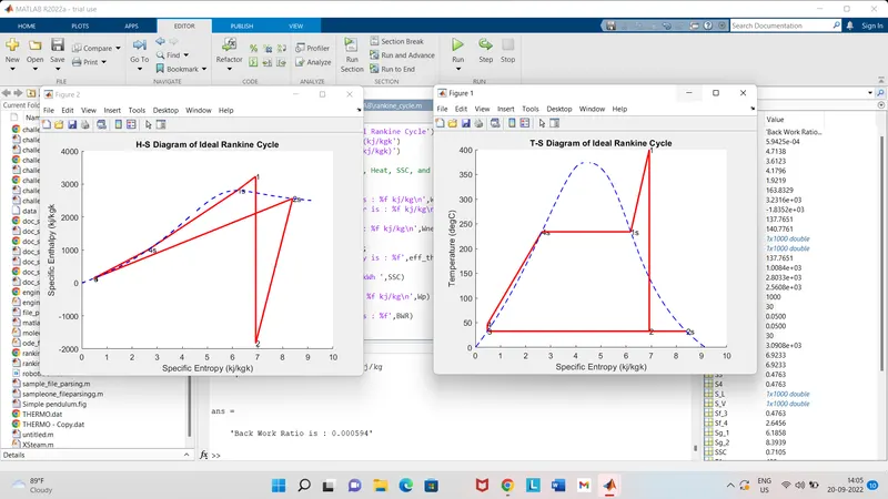
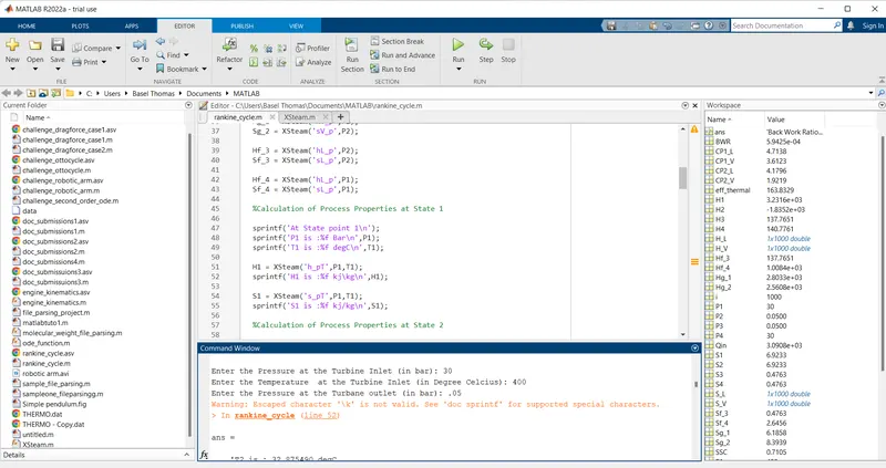
ERROR

Incorrectly put \ instead of / in kj/kg

CORRECTIONS

Accuractly put / by removing \ sign
EXPLANATION OF CODE

clear all
close all
clc    - for clearing existing windows

% Printing Introduction

sprintf(' RANKINE CYCLE SIMULATOR \n\n') - sprintf is used to return the data in the xsteam file into a  matlab string variable. And to print Rankine Cycle Simulator, \n are literal text that are associated with sprintf command.
sprintf('1-2 is Isentropic Expansion in the Turbine\n') -  sprintf is used to return the data in the xsteam file into a  matlab string variable. And to print 1-2 Isentropic expansion in the turbine, \n are literal text that are associated with sprintf command.

sprintf('2-3 is Constant Pressure Heat Rejection by the Condenser\n') -   sprintf is used to return the data in the xsteam file into a  matlab string variable. And to print 2-3 Constant Pressure Heat Rejection by the Condenser, \n are literal text that are associated with sprintf command.
sprintf('3-4 is Isentropic Compression in pump\n') - sprintf is used to return the data in the xsteam file into a  matlab string variable. And to print 3-4 Isentropic Compression in pump, \n are literal text that are associated with sprintf command.
sprintf('4-1 is Constant Pressure Heat Addition by the Boiler\n\n') - sprintf is used to return the data in the xsteam file into a  matlab string variable. And to print 4-1 Constant Pressure Heat Addition by the Boiler, \n are literal text that are associated with sprintf command.

% User Inputs
P1 = input('Enter the Pressure at the Turbine Inlet (in bar): '); - command for showing in the command window for the user to put specific values for the inlet pressure (P1)
T1 = input('Enter the Temperature  at the Turbine Inlet (in Degree Celcius): '); - command for showing in the command window for the user to put specific values for the inlet temperature (T1)
P2 = input('Enter the Pressure at the Turbane outlet (in bar): '); - command for showing in the command window for the user to put specific values for the outlet pressure (P2)

sprintf('   RESULT\n'); - sprintf command for showing the results in a string variable

%Calculation of Cp values at P1 & P2 for saturated liquid & vapour

CP1_L = XSteam('CpL_p',P1); - for calculating the specific isobaric heat capacities at p1 & p2. cp1_L is the saturated liquid heat capacity at  Pressure inlet 1
CP1_V = XSteam('CpV_p',P1); - cp1_v is the saturated vapour heat capacity at pressure inlet 1
CP2_L = XSteam('CpL_p',P2); - cp2_L is the saturated liquid heat capacity at  Pressure ioutlet 2
CP2_V = XSteam('CpV_p',P2); - cp2_v is the saturated vapour heat capacity at pressure outlet 2

% Calculation of Saturation Temperature at P1 & P2
Tsat_P1 = XSteam('Tsat_p',P1); Tsat_p1 is the saturation temperature at pressure inlet 1
Tsat_P2 = XSteam('Tsat_p',P2); Tsat_p2 is the saturation temperature at pressure outlet  2

% Calculation of saturation of Enthalpy & Entropy at saturation points
Hg_1 = XSteam('hV_p',P1); - Hg_1 is the saturated vapour enthalpy at pressure inlet 1
Sg_1 = XSteam('sV_p',P1); - Sg_1 is the saturated vapour entropy at pressure inlet 1

Hg_2 = XSteam('hV_p',P2); - Hg_2 is the saturated vapour enthalpy at pressure outlet 2
Sg_2 = XSteam('sV_p',P2); - Sg_2 is the saturated vapour entropy at pressure outlet 2

Hf_3 = XSteam('hL_p',P2); - Hf_3 is the saturated liquid enthalpy at pressure outlet 2
Sf_3 = XSteam('sL_p',P2); - Sf_3 is the saturated liquid entropy at pressure outlet 2

Hf_4 = XSteam('hL_p',P1); - Hf_4 is the saturated liquid enthalpy at pressure inlet 1
Sf_4 = XSteam('sL_p',P1); - Sf_4 is the saturated liquid entropy at pressure inlet 1

%Calculation of Process Properties at State 1

sprintf('At State point 1\n'); - sprintf command for returning string variable as at state point 1
sprintf('P1 is :%f Bar\n',P1); - command for showing p1 value as of a string variable printing in bar
sprintf('T1 is :%f degC\n',T1); - command for showing T1 value as of  a string variable printing in degree celcius

H1 = XSteam('h_pT',P1,T1); - H1 is the enthalpy as a function of pressure and temperature
sprintf('H1 is :%f kj/kg\n',H1); - for printing of H1 as a string variable

S1 = XSteam('s_pT',P1,T1); - S1 is the entropy as a function of pressure and temperature
sprintf('S1 is :%f kj/kg\n',S1); - for printing of S1 as a string variable


%Calculation of Process Properties at State 2

sprintf('At State point 2\n'); - sprintf command for returning string variable as at state point 2
sprintf('P2 is :%f Bar\n',P2); - command for showing p2 value as of a string variable printing in bar

S2 = S1;
sprintf('S2 is :%f kj/kg\n',S2); -  for printing of S2 as a string variable


% calculating value of x

if(S2<=Sg_2) if statement is used to specify a condition that S2 is lesser than or equal to sg_2
    X2 = (S2 - Sf_3) / (Sg_2-Sf_3); then x is the difference between s2 & sf3
else - otherwise
    X2=1; - the value of x2 is 1
end for ending the condition
sprintf('X2 is :%f \n', X2); - for printing the value of x2

% calculating value of T2

if(X2<1) - if statement is used to specify a condition that x2 is lesser than 1
    T2=Tsat_P2; - t2 value is equal to saturated temp at p2
else - otherwise
    %S2=Sg_2+CP2_V*(log(T2/Tsat_P2)) - equation for calculating s2
    T2=(Tsat_P2+273.15)*exp((S2-Sg_2)/CP2_V); - equation for finding t2
    T2=T2-273.15; - hence we can find the values for t2
end - for ending the statement
sprintf('T2 is : %f degC \n',T2) - command for printing the t2 value
if(X2<1) - if statement is used to specify a condition that x2 is lesser than 1 -
    H2 = Hf_3 + X2*(Hf_3-Hg_2); - equation for finding h2
else - otherwise
    H2=XSteam('h_pT',P2,T2); if h2 value is greater than 1, then use this equation
end - for ending the statement
sprintf('H2 is : %f kj/kg\n\n',H2)

%Calculation of Process Properties at State 3

sprintf('At state point 3\n') - sprintf command for returning string variable as at state point 3

P3=P2;
sprintf('P3 is : %f Bar\n', P3) - for printing the value of p3

V3 = XSteam('vL_p', P3); v3 is the vapourised liquid pressure 3

T3 = Tsat_P2; - t3 is the saturated temperature at point 2
sprintf('T3 is : %f degC\n', T3) - for printing the t3 value by returning in string variable as of degree celsius

H3 = Hf_3; - value of h3 is hf_3
sprintf('H3 is : %f kj/kg\n\n',H3) - for printing the h3 value by returning in string variable as of kj\kg

S3 = Sf_3; - vallue of s3 is sf_3
sprintf('S3 is : %f kj/kgk\n\n', S3) - for printing the s3 value by returning in string variable as of kj\kg

%Calculation of Process Properties at State 4

sprintf('At state point 4\n') - sprintf command for returning string variable as at state point 4

P4 = P1;
sprintf('P4 is : %f Bar\n', P4) - for printing the p4 value

S4 = S3;
sprintf('S4 is : %f kj/kgk\n\n', S4) -for printing the t3 value by returning in string variable as of degree celsius

Wp = V3 * (P4-P3) * 100; - equation for finding work done by pump
H4 = Wp + H3; for finding the entropy at point 4
sprintf('H4 is : %f kj/kg\n',H4) - for printing the value of H4

T4 = (Tsat_P1+273.15)/(exp((Sf_4-S4)/CP1_L));
T4 = T4 - 273.15; - equations for finding temperature at point 4
sprintf('T4 is : %f Deg celsius \n\n', T4) - for printing the value of T4

%Calculation & plotting saturation Liquid and Vapour lines

temp = linspace(1, T1, 1000); - for creating a matrix array of 1 to t1 with 1000 limits
for i = 1:length(temp) - i stores the values for length of temperature, for loop used for the reccuring operations for finding the entropy and enthalpy values with respect to temperature
    H_L(i) = XSteam('hL_T', temp(i)); - liquid enthalpy values may stored in the i from xsteam file of enthalpy liquid temperature
    H_V(i) = XSteam('hV_T', temp(i)); - vapour enthalpy values may stored in the i from xsteam file of enthalpy vapour temperature
    S_L(i) = XSteam('sL_T', temp(i)); - liquid entropy values may stored in the i from xsteam file of entropy liquid temperature
    S_V(i) = XSteam('sV_T', temp(i)); - vapour entropy values may stored in the i from xsteam file of entropy vapour temperature

end

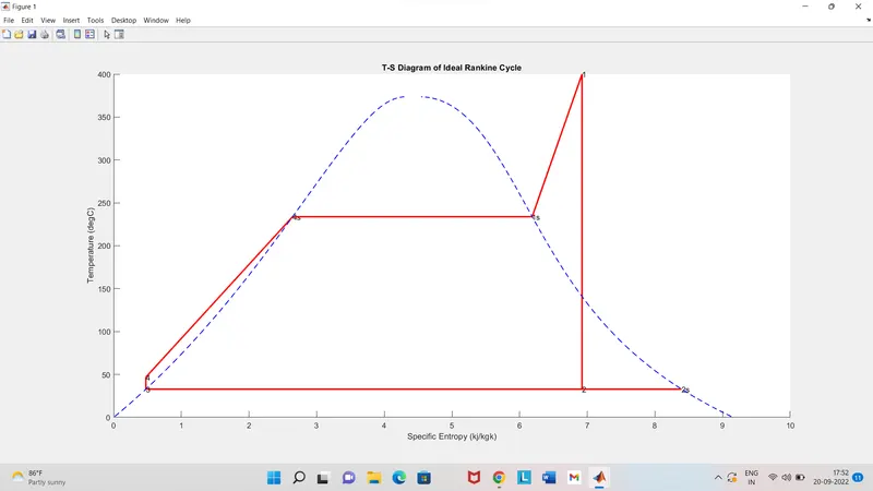
% PLOTTING T-S DIAGRAM

figure(1)- for showing the diagram as figure 1
hold on - for holding the figure without overwritting
plot([S1 S2],[T1 T2], 'r','LineWidth',2) - for plotting s1,s2 and t1 t2 with red color of linewidth 2
text(S1,T1,'1') - for showing the text s1,t1 as 1st connection
text(S2,T2,'2') - for showing the text s2,t2 as 2nd connection
plot([S2 Sg_2],[T2 Tsat_P2],'r','LineWidth',2) - for plotting s2, sg_2 and t2, tsat_p2 with red color of linewidth 2
text(Sg_2,Tsat_P2,'2s') -for showing the text sg_2, tsat_p2 as 2s connection
plot([Sg_2 S3],[Tsat_P2 T3],'r','LineWidth',2) -  for plotting sg_2,s3 and tsat_p2,t3 with red color of linewidth 2
text(S3,T3,'3') - for showing the text s3,t3 as 3rd connection
plot([S3 S4],[T3 T4], 'r','LineWidth',2) - for plotting s3,s4 and t3, t4 with red color of linewidth 2
text(S4,T4,'4') - for showing the text s4,t4 as 4th connection
plot([S4 Sf_4],[T4 Tsat_P1],'r','LineWidth',2) - for plotting s4,sf_4 and t4,tsat_p1 with red color of linewidth 2
text(Sf_4,Tsat_P1,'4s') - for showing the text sf_4,tsat_p1 as 4s connection
plot([Sf_4,Sg_1],[Tsat_P1 Tsat_P1],'r','LineWidth',2) - for plotting sf_4,sg_1 and tsat_p1 with red color of linewidth 2
text(Sg_1, Tsat_P1,'1s') - for showing the text sg_1,tsat_p1 as 1s connection
plot([Sg_1 S1], [Tsat_P1 T1], 'r','LineWidth',2) - for plotting s1,sg_1 and tsat_p1,t1 with red color of linewidth 2
plot(S_L, temp, 'b', 'LineStyle','--','LineWidth',1) - for plotting s_l vs temp dia with a linestyle '--'& linewidth of 1 mm of color blue
plot(S_V, temp, 'b', 'LineStyle','--','LineWidth',1) - for plotting s_v vs temp dia with a linestyle '--'& linewidth of 1 mm of color blue

title('T-S Diagram of Ideal Rankine Cycle') - for showing the title for diagram  as T-S Diagram of Ideal Rankine Cycle
ylabel('Temperature (degC)') - for labebelling y axis as temp (degC)
xlabel('Specific Entropy (kj/kgk)') - for labelling x axis as specific entropy kj\kgk

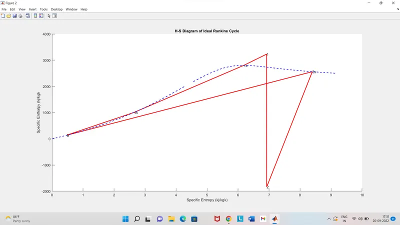
% Plotting H-S Plot

figure(2) - for showing the diagram as figure 2
hold on - for holding the figure without overwritting
plot([S1 S2],[H1 H2], 'r','LineWidth',2) - for plotting s1,s2 and h1 h2 with red color of linewidth 2
text(S1,H1,'1') - for showing the text s1,h1 as 1st connection
text(S2,H2,'2') - for showing the text s1,h1 as 2nd connection
plot([S2 Sg_2], [H2 Hg_2],'r','LineWidth',2) - plotting s2, sg_2 and h2, hg_2 with red color of linewidth 2
text(Sg_2,Hg_2,'2s') - for showing the text sg_2,hg_2 as 2s connection
plot([Sg_2 S3],[Hg_2 H3],'r','LineWidth',2) - plotting sg_2,s3 and hg_2,h3 with red color of linewidth 2
text(S3,H3,'3') - for showing the text s3,h3 as 3rd connection
plot([S3 S4],[H3 H4], 'r','LineWidth',2) - for plotting s3,s4 and h3 h4 with red color of linewidth 2
text(S4,H4,'4') - for showing the text s4,h4 as 4th connection
plot([S4 Sf_4],[H4 Hf_4],'r','LineWidth',2) - for plotting s4,sf_4 and h4,hf_4 with red color of linewidth 2
text(Sf_4,Hf_4,'4s') - for showing the text sf4,hf4 as 4s connection
plot([Sf_4,Sg_1],[Hf_4 Hg_1],'r','LineWidth',2) - for plotting sf_4,sg_1 and hf_4,hg_1 with red color of linewidth 2
text(Sg_1, Hg_1,'1s') - for showing the text sg_1,hg_4 as 1s connection
plot([Sg_1 S1], [Hg_1 H1], 'r','LineWidth',2) - for plotting sg_1,s1 and hg_1,h1 with red color of linewidth 2
plot(S_L, H_L,'b','LineStyle','--','LineWidth',1.5) -  for plotting s_l vs h_l dia with a linestyle '--'& linewidth of 1.5 mm of color blue
plot(S_V, H_V,'b','LineStyle','--','LineWidth',1.5) -   for plotting s_v vs h_v dia with a linestyle '--'& linewidth of 1.5 mm of color blue


title('H-S Diagram of Ideal Rankine Cycle') - for showing the title for diagram  as H-S Diagram of Ideal Rankine Cycle
ylabel('Specific Enthalpy (kj/kgk') - for labebelling y axis as Specific Enthalpy (kj/kgk)
xlabel('Specific Entropy (kj/kgk)') - for labelling x axis as Specific Entropy (kj/kgk)

% Calculation of Work Done, Heat, SSC,Themal Efficiency &  BWR

Wt = H1-H2; - equation for finding work done by turbine
sprintf('Work by turbine is : %f kj/kg\n',Wt) - for printing the Wt values which sprintf return it as astring variable from the XSteam file
sprintf('Work by compressor is : %f kj/kg\n',Wp)
Wnet = Wt - Wp; - net work output equation
sprintf('Net Work done is : %f kj/kg\n',Wnet) - command for printing the valuue of work output which sprintf return it as astring variable from the XSteam file
Qin = H1 - H4; equation for finding the heat
eff_thermal = Wnet*100/Qin; - equation for finding the thermal efficiency
sprintf('Thermal Efficiency is : %f',eff_thermal); disp('%') - for printing the thermal efficiency in % which sprintf return it as astring variable from the XSteam file
SSC = 3600/Wt; equation for finding the specific steam consumption
sprintf('S.S.C is : %f kg/kWh ',SSC) - for the printing the value of ssc which sprintf return it as astring variable from the XSteam file
Wp = H4-H3; equation for finding the workdone by pump
sprintf('Work by pump is : %f kj/kg\n',Wp) - for printing the wr value which sprintf return it as astring variable from the XSteam file
BWR = Wp/Wt; equation for finding BWR
sprintf('Back Work Ratio is : %f',BWR) - for printing the WBR values which sprintf return it as astring variable from the XSteam file
% Rankine Cycle Simulator
clear
close all
clc

% Printing Introduction

sprintf(' RANKINE CYCLE SIMULATOR \n\n')
sprintf('1-2 is Isentropic Expansion in the Turbine\n')
sprintf('2-3 is Constant Pressure Heat Rejection by the Condenser\n')
sprintf('3-4 is Isentropic Compression in pump\n')
sprintf('4-1 is Constant Pressure Heat Addition by the Boiler\n\n')

% User Inputs
P1 = input('Enter the Pressure at the Turbine Inlet (in bar): ');
T1 = input('Enter the Temperature  at the Turbine Inlet (in Degree Celcius): ');
P2 = input('Enter the Pressure at the Turbane outlet (in bar): ');

sprintf('   RESULT\n');

%Calculation of Cp values at P1 & P2 for saturated liquid & vapour

CP1_L = XSteam('CpL_p',P1);
CP1_V = XSteam('CpV_p',P1);
CP2_L = XSteam('CpL_p',P2);
CP2_V = XSteam('CpV_p',P2);

% Calculation of Saturation Temperature at P1 & P2
Tsat_P1 = XSteam('Tsat_p',P1);
Tsat_P2 = XSteam('Tsat_p',P2);

% Calculation of saturation of Enthalpy & Entropy at saturation points
Hg_1 = XSteam('hV_p',P1);
Sg_1 = XSteam('sV_p',P1);

Hg_2 = XSteam('hV_p',P2);
Sg_2 = XSteam('sV_p',P2);

Hf_3 = XSteam('hL_p',P2);
Sf_3 = XSteam('sL_p',P2);

Hf_4 = XSteam('hL_p',P1);
Sf_4 = XSteam('sL_p',P1);

%Calculation of Process Properties at State 1

sprintf('At State point 1\n');
sprintf('P1 is :%f Bar\n',P1);
sprintf('T1 is :%f degC\n',T1);

H1 = XSteam('h_pT',P1,T1);
sprintf('H1 is :%f kj/kg\n',H1);

S1 = XSteam('s_pT',P1,T1);
sprintf('S1 is :%f kj/kg\n',S1);

%Calculation of Process Properties at State 2

sprintf('At State point 2\n');
sprintf('P2 is :%f Bar\n',P2);

S2 = S1;
sprintf('S2 is :%f kj/kg\n',S2);

% calculating value of x

if(S2<=Sg_2)
    X2 = (S2 - Sf_3) / (Sg_2-Sf_3);
else
    X2=1;
end
sprintf('X2 is :%f \n', X2);

% calculating value of T2

if(X2<1)
    T2=Tsat_P2;
else
    %S2=Sg_2+CP2_V*(log(T2/Tsat_P2))
    T2=(Tsat_P2+273.15)*exp((S2-Sg_2)/CP2_V);
    T2=T2-273.15;
end
sprintf('T2 is : %f degC \n',T2)
if(X2<1)
    H2 = Hf_3 + X2*(Hf_3-Hg_2);
else
    H2=XSteam('h_pT',P2,T2);
end
sprintf('H2 is : %f kj/kg\n\n',H2)

%Calculation of Process Properties at State 3

sprintf('At state point 3\n')

P3=P2;
sprintf('P3 is : %f Bar\n', P3)

V3 = XSteam('vL_p', P3);

T3 = Tsat_P2;
sprintf('T3 is : %f degC\n', T3)

H3 = Hf_3;
sprintf('H3 is : %f kj/kg\n\n',H3)

S3 = Sf_3;
sprintf('S3 is : %f kj/kgk\n\n', S3)

%Calculation of Process Properties at State 4

sprintf('At state point 4\n')

P4 = P1;
sprintf('P4 is : %f Bar\n', P4)

S4 = S3;
sprintf('S4 is : %f kj/kgk\n\n', S4)

Wp = V3 * (P4-P3) * 100;
H4 = Wp + H3;
sprintf('H4 is : %f kj/kg\n',H4)

T4 = (Tsat_P1+273.15)/(exp((Sf_4-S4)/CP1_L));
T4 = T4 - 273.15;
sprintf('T4 is : %f Deg celsius \n\n', T4)

%Calculation & plotting saturation Liquid and Vapour lines

temp = linspace(1, T1, 1000);
for i = 1:length(temp)
    H_L(i) = XSteam('hL_T', temp(i));
    H_V(i) = XSteam('hV_T', temp(i));
    S_L(i) = XSteam('sL_T', temp(i));
    S_V(i) = XSteam('sV_T', temp(i));
end

% PLOTTING T-S DIAGRAM

figure(1)
hold on
plot([S1 S2],[T1 T2], 'r','LineWidth',2)
text(S1,T1,'1')
text(S2,T2,'2')
plot([S2 Sg_2],[T2 Tsat_P2],'r','LineWidth',2)
text(Sg_2,Tsat_P2,'2s')
plot([Sg_2 S3],[Tsat_P2 T3],'r','LineWidth',2)
text(S3,T3,'3')
plot([S3 S4],[T3 T4], 'r','LineWidth',2)
text(S4,T4,'4')
plot([S4 Sf_4],[T4 Tsat_P1],'r','LineWidth',2)
text(Sf_4,Tsat_P1,'4s')
plot([Sf_4,Sg_1],[Tsat_P1 Tsat_P1],'r','LineWidth',2)
text(Sg_1, Tsat_P1,'1s')
plot([Sg_1 S1], [Tsat_P1 T1], 'r','LineWidth',2)
plot(S_L, temp, 'b', 'LineStyle','--','LineWidth',1)
plot(S_V, temp, 'b', 'LineStyle','--','LineWidth',1)

title('T-S Diagram of Ideal Rankine Cycle')
ylabel('Temperature (degC)')
xlabel('Specific Entropy (kj/kgk)')

% Plotting H-S Plot

figure(2)
hold on
plot([S1 S2],[H1 H2], 'r','LineWidth',2)
text(S1,H1,'1')
text(S2,H2,'2')
plot([S2 Sg_2], [H2 Hg_2],'r','LineWidth',2)
text(Sg_2,Hg_2,'2s')
plot([Sg_2 S3],[Hg_2 H3],'r','LineWidth',2)
text(S3,H3,'3')
plot([S3 S4],[H3 H4], 'r','LineWidth',2)
text(S4,H4,'4')
plot([S4 Sf_4],[H4 Hf_4],'r','LineWidth',2)
text(Sf_4,Hf_4,'4s')
plot([Sf_4,Sg_1],[Hf_4 Hg_1],'r','LineWidth',2)
text(Sg_1, Hg_1,'1s')
plot([Sg_1 S1], [Hg_1 H1], 'r','LineWidth',2)
plot(S_L, H_L,'b','LineStyle','--','LineWidth',1.5)
plot(S_V, H_V,'b','LineStyle','--','LineWidth',1.5)

title('H-S Diagram of Ideal Rankine Cycle')
ylabel('Specific Enthalpy (kj/kgk')
xlabel('Specific Entropy (kj/kgk)')

% Calculation of Work Done, Heat, SSC, and Efficiency

Wt = H1-H2;
sprintf('Work by turbine is : %f kj/kg\n',Wt)
sprintf('Work by compressor is : %f kj/kg\n',Wp)
Wnet = Wt - Wp;
sprintf('Net Work done is : %f kj/kg\n',Wnet)
Qin = H1 - H4;
eff_thermal = Wnet*100/Qin;
sprintf('Thermal Efficiency is : %f',eff_thermal); disp('%')
SSC = 3600/Wt;
sprintf('S.S.C is : %f kg/kWh ',SSC)
Wp = H4-H3;
sprintf('Work by pump is : %f kj/kg\n',Wp)
BWR = Wp/Wt;
sprintf('Back Work Ratio is : %f',BWR)


RANKINE CYCLE COMMAND WINDOW RESULTS

' RANKINE CYCLE SIMULATOR

     '


ans =

    '1-2 is Isentropic Expansion in the Turbine
     '


ans =

    '2-3 is Constant Pressure Heat Rejection by the Condenser
     '


ans =

    '3-4 is Isentropic Compression in pump
     '


ans =

    '4-1 is Constant Pressure Heat Addition by the Boiler

     '

Enter the Pressure at the Turbine Inlet (in bar): 30
Enter the Temperature  at the Turbine Inlet (in Degree Celcius): 400
Enter the Pressure at the Turbane outlet (in bar): .05

ans =

    'T2 is : 32.875490 degC
     '


ans =

    'H2 is : -1835.177974 kj/kg

     '


ans =

    'At state point 3
     '


ans =

    'P3 is : 0.050000 Bar
     '


ans =

    'T3 is : 32.875490 degC
     '


ans =

    'H3 is : 137.765119 kj/kg

     '


ans =

    'S3 is : 0.476254 kj/kgk

     '


ans =

    'At state point 4
     '


ans =

    'P4 is : 30.000000 Bar
     '


ans =

    'S4 is : 0.476254 kj/kgk

     '


ans =

    'H4 is : 140.776056 kj/kg
     '


ans =

    'T4 is : 46.846863 Deg celsius

     '


ans =

    'Work by turbine is : 5066.749001 kj/kg
     '


ans =

    'Work by compressor is : 3.010937 kj/kg
     '


ans =

    'Net Work done is : 5063.738064 kj/kg
     '

%

ans =

    'S.S.C is : 0.710515 kg/kWh '


ans =

    'Work by pump is : 3.010937 kj/kg
     '


ans =

    'Back Work Ratio is : 0.000594'

>>