Week 5 - Genetic Algorithm
Week 5 - Genetic Algorithm
Question
Try to understand the concept of the genetic algorithm by referring to various sources before you attend this challenge. Look out for information regarding the stalagmite function and ways to optimise it.
- Write a code in MATLAB to optimise the stalagmite function and find the global maxima of the function.
- Clearly explain the concept of genetic algorithm in your own words and the syntax for 'ga' in MATLAB in your report.
- Make sure that your code gives the same output, even if it is made to run several times.
- Plot graphs for all 3 studies and F maximum Vs. No. of iterations. Title and axes labels are a must legends could be shown if necessary.
The presentation of your code will be taken into consideration while grading. Labelling sections of your code is appreciated.
Content expected in the report.
- Step-wise explanation of your code.
- Mention the errors while programming.
- Steps were taken to overcome those errors.
- Screenshots showing errors thrown in the command window.
Under references, mention the literature or online material you have used during research.
Answers
Introduction To Genetic Algorithm (GA)
Nature has been a great source of inspiration to all mankind. Genetic Algorithms (GA) are search-based algorithms based on the concepts of natural selection and genetics.
GAs were developed by John Holland and his students and colleagues at the University of Michigan, most notably David E. Goldberg and have since been tried on various optimization problems with a high degree of success.
We can apply the GA to solve problems not well-suited for standard optimization algorithms including problems in which the objective function is discontinued, non-differentiable, stochastic, or highly non-linear.
The GA differs from a classical, derivative-based, optimization algorithm in two ways,
| Classical Algorithm | Genetic Algorithm |
| Generates a single point on each iteration. The sequence of points approaches an optimal solution. | Generates a population of points at each iteration. The best point in the population approaches an optimal solution |
| Selects the next point in the sequence by a deterministic computation. | Selects the next population by computation which uses random number generators. |
Optimization
Optimization is the process of making something better. In any process, we have a set of inputs.
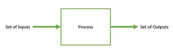
Optimization refers to finding the values of inputs in such a way that we get the 'best' output values. The definition of 'best' varies from problem to problem, but in mathematical terms, it refers to maximizing or minimizing one or more objective functions, by varying the input parameters.
The set of all possible solutions or values the inputs can take makes up the search space. In this search space, lies a point or a set of points that gives the optimal solution. Optimization aims to find that point or set of points in the search space.
Genetic Algorithm (GA)
A genetic algorithm (GA) solves both constrained and unconstrained optimization problems based on a natural selection process that mimics biological evolution. The algorithm repeatedly modifies the population of individual solutions. At each step, the GA randomly selects individuals from the current population and uses them as parents to produce children for the next generation. Over successive generations, the population "evolves" towards the optimal solution.
In other words, the Genetic Algorithm (GA) is a search-based optimization technique based on genetic and natural selection principles. It is frequently used to find optimal or near-optimal solutions to difficult problems that otherwise would take a lifetime to solve. It is frequently used to solve optimization problems in research and machine learning.
Figure 1
In GAs, we have a pool or population of possible solutions to the given problem. These solutions then undergo recombination and mutation (like in natural genetics), producing new children and the process is repeated over various generations. Each individual is assigned a fitness value (based on its objective function value) and the fitter individuals are given a higher chance to mate and yield more 'fitter' individuals. This is in line with the 'Darwin Theory Of Survival Of The Fittest'.
In this way, we keep 'evolving' better individuals or solutions over generations, till we reach a stopping criterion.
GAs are sufficiently randomized in nature, but they perform much better than random local search (in which we just try various random solutions, keeping track of the best so far), as they exploit historical information as well.
Genetic Algorithm (GA) - Why We Need
GAs can deliver a 'good-enough' solution 'fast enough', and it makes GAs more attractive for use in solving optimization problems. The reasons why GAs are needed are as follows
- Solving difficult problems:- Solving large sets of problems that even the most powerful computing systems take a very long time to solve. GAs are very capable and efficient tools to provide usable near-optimal solutions in a short period.
- Failure of gradient-based methods
- Getting a good solution as fast.
Genetic Algorithm (GA) - Basic Terminologies
- Population:- Subset of all possible (encoded) solutions to the given problem.
- Chromosome:- It is one such solution to the given problem.
- Gene:- One element position of a chromosome
- Allele:- Value a gene takes for a particular chromosome.
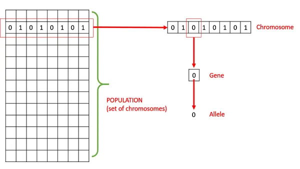
Figure 2 - Genotype:- Population in the computation space, where the solutions are represented in a way that can be easily understood and manipulated using a computing system.
- Phenotype:- Population in the actual real solution space in which solutions are represented in a way they are represented in real-world situations.
- Decoding:- Process of transforming a solution from genotype to the phenotype space.
- Encoding:- Process of transforming from the phenotype to the genotype.
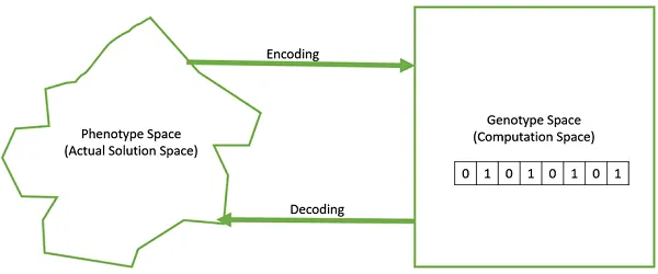
Figure 3 - Fitness Function:- A function that takes the solution as input and produces suitability of the solution as the output.
- Genetic Operators:- These alter the genetic composition of the offspring. These include crossover, mutation, selection, etc.
Genetic Algorithm (GA) - Basic Structure
Starting with an initial population (which may be generated at random or seeded by other heuristics), select parents from this population for mating. Apply crossover and mutation operators on the parents to generate new offspring and finally these offspring replace the existing individuals in the population and the process repeats. In this way, GAs try to mimic human evolution in some context.
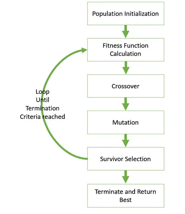
Figure 4
A generalized pseudocode for the GA is mentioned below.
FUNCTION GA()

   INITIALIZE Population
   FIND The Fitness Of The Population

  WHILE Termination Criteria Is Reached

       DO Parent selection
       DO Crossover With Probability PC
       DO Mutation With Probability PM
       DO Decoding
       DO Fitness Calculation
       DO Survivor Selection

       FIND Best Offspring

       OUTPUT Best Offspring

  ENDWHILE
Genetic Algorithm (GA) - How It Works
The following outline summarizes how GA works.
- Creating a random initial population.
- Creates a sequence of new populations. At each step, the algorithm uses the individuals in the current generation to create the next population. To create the new population, the algorithm performs the following steps.
a. Scores each member of the current population by computing its fitness value known as 'raw fitness scores'.
b. Scales the raw fitness scores to convert them into a more usable range of values known as 'expectation values'.
c. Select members called as 'parents' based on their expectations.
d. Some of the individuals in the current population who have lower fitness are chosen as elite. These elite individuals are passed on to the next population.
e. Produces children from parents. Children are produced either by making random changes to a single parent (Mutation) or by combining vector entities of a pair of parents (Crossover).
f. Replaces the current population with the children to form the next population. - The algorithm stops when one of the criteria is met.
- The algorithm takes modified steps for linear and integral constraints.
- The algorithm is further modified for nonlinear constraints.
Genetic Algorithm (GA) - Advantages
- Does not require any derivative information (which may not be available for many real-world problems.)
- Is faster and more efficient as compared to the traditional methods.
- Has very good parallel capabilities.
- Optimizes both continuous and discrete functions and also multi-objective problems.
- Provides a list of 'good' solutions and not just one solution.
- Always gets an answer to the problem, which gets better over time.
- Useful when the search space is very large and there are a large number of parameters involved.
Genetic Algorithm (GA) - Limitations
- Not suited for all problems, especially problems that are simple and for which derivative information is available.
- The fitness value is calculated repeatedly which might be computationally expensive for some cases.
- Being stochastic, there are no guarantees on the optimally or the quality of the solution.
- If not implemented properly, the GA may not converge to the optimal solution.
Function 'ga' - Matlab Syntax And Descriptions
The function 'ga' in MATLAB uses GA to find a local minimum of a function. It can optimize a function with or without linear or nonlinear constraints, and accept extra parameters for the objective function and nonlinear constraints.
Different types of 'ga' functions and their syntax are given below.
1.
x = ga(fun,nvars)Finds a local unconstrained minimum 'x' to the objective function, 'fun'.
- fun:- Objective function
- nvars:- Number of design variables.
2.
x = ga(fun,nvars,A,b)Finds a local minimum 'x' to 'fun', subject to the linear inequalities `A"*"x<=b`. Function 'ga' evaluates the matrix product `A"*"x` as if x is transported (`A"*"x'`)
- A, b:- Matrices that define the linear inequalities `A"*"x<=b`.
3.
x = ga(fun,nvars,A,b,Aeq,beq)Finds a local minimum 'x' to 'fun', subject to the linear inequalities `A_"eq" "*"x=b_"eq"` and `A"*"x<=b`. Set A=[] and b=[] if no linear inequalities exist. ga evaluates the matrix product `A_"eq""*"x and if transposed `A_"eq""*"x '`
- Aeq and beq:- Matrices that define the linear equalities `A_"eq" "*"x=b_"eq"`
4.
x = ga(fun,nvars,A,b,Aeq,beq,lb,ub)Defines a set of lower and upper bounds on the design variables x, so that a solution is found in the range `lb<=x<=ub`. Set Aeq=[] and beq=[] if no linear equalities exist.
- lb and ub:- Vectors that define the lower and upper bounds.
5.
x = ga(fun,nvars,A,b,Aeq,beq,lb,ub,nonlcon)Subjects the minimization to the constraints defined in 'nonlcon'. The function accepts x and returns C and Ceq, representing the nonlinear inequalities and equalities respectively. The ga minimizes the objective function 'fun' such that `C(x)<=0 and C_"eq"=0`. Set lb =[] and ub=[] if no bounds exist`
- nonlcon:- Function handle that defines the nonlinear constraints.
6.
x = ga(fun,nvars,A,b,Aeq,beq,lb,ub,nonlcon,options)Minimizes with the default optimization parameters replaced by values in 'options'. Set 'nonlcon'= [] if no nonlinear constraints exist.) Create 'options' using 'optimoptions'.
- Options:- Structure that contains options for the optimization process such as population size, mutation and crossover functions and termination criteria.
7.
x = ga(fun,nvars,A,b,Aeq,beq,lb,ub,nonlcon,intcon)

% OR

x = ga(fun,nvars,A,b,Aeq,beq,lb,ub,nonlcon,intcon,options)
Requires that the variables listed in 'intcon' take integer values.
- intcon:- Vector that defines the indices of integer variables.
8.
[x,fval] = ga (___)For any previous input arguments, also returns 'fval', the value of the fitess function at x.
- fval:- Value of fitness function at x.
9.
[x,fval,exitflag,output] = ga(___)Also returns 'exitflag' an integer identifying the reason the algorithm terminated and 'output', a structure that contains output from each generation and other information about the performance of an algorithm.
- exitflag:- Integer identifying the reason the algorithm terminated
- output:- A structure that contains output from each generation and other information about the performance of an algorithm.
10.
[x,fval,exitflag,output,population,scores] = ga(___)Returns a matrix 'population' whose rows are the final population and a vector 'scores' the scores of the final population.
- population:- A matrix whose rows are the final population
- scores:- A vector that scores the final population.
MATLAB Code
1. Stalagmite Function
We need to create a function that has a single variable 'IP_Vector'.Name the function as "Stalagmite". The function gives us the output of [F] by following a set of equations,
`F1x=(sin((5.1*pi*x)+0.5))^6`
`F1y=(sin((5.1*pi*y)+0.5))^6`
`F2x=exp(-4*ln(2)*((x-0.067)^2/0.64))`
`F2y=exp(-4*ln(2)*((y-0.067)^2/0.64))`
`F1=F1x*F1y*F2x*F2y`
`F=-F1`
The -F value gives the global maxima of the given stalagmite function. The syntax for the function is given below. Please note that
- x = IP_Vector(1)
- y = IP_Vector(2)
% Starting the function initiation. The variable is "IP_Vector"
% F(x,y) = (F1x)*(F2x)*(F1y)*(F2y)

function [F]=Stalagmite (IP_Vector)

         F1X = (sin((5.1.*pi.*IP_Vector(1))+0.5)).^6;

         F1Y = (sin((5.1.*pi.*IP_Vector(2))+0.5)).^6;

         F2X = exp((-4*log(2)*((IP_Vector(1)-0.0667)./0.64).^2));

         F2Y = exp((-4*log(2)*((IP_Vector(2)-0.0667)./0.64).^2));

         F1 = F1X*F1Y*F2X*F2Y;

         F = -F1;

end
2. Matlab Code
- Create two 1D arrays X and Y from 0 to 0.6 and the array has a total of 150 variables. From these 1D arrays, we need to create a 2D array with the help of a 'meshgrid'. Create a variable 'N' that stores the total number of iterations.
- Starting the timer for the evaluation of stalagmite. function.
- Initiate a FOR loop, with a length of 'XX', and inside of that loop, initiate another FOR loop for the length of 'YY'. Using those FOR loops find the value of 'F' for every value of 'i' and 'j'.
- Select the figure window. Plot the 3D graph between 'XX' vs 'YY' vs '-F'. Remove mesh from the plot by using the 'shading interp' command. Manage the plot by naming axes and titles.
- After the evaluation, end the timer and store the value in a variable 'Stalagmite_Evaluation_Time'.
- For case 1, we need to find the solution for the optimisation problem by using the unbounded inputs. Initiate the timer for recording the time taken for the analysis.
- Initiate a FOR loop for the number of iterations, 100. By using the following syntax, we need to find the best values for the problem.
x = ga(fun,nvars)
Here 'fun' indicates the 'GA' function, 'Stalagmite' and 'nvars' stands for the number of design variables,2. The code gives two outputs 'Inputs' and 'Fopt_1'. Then list out the values for the x (Xopt_1) and y (Yopt_1) axis from the values of the first and second position of variable 'Inputs'. End the FOR loop. - End the timer. Save the total time taken into a variable 'Analysis_1_Running_Time'.
- Create a new figure window. Within the figure, create a subplot and plot the Stalagmite Function between 'XX' vs 'YY' vs '-F'. Remove mesh from the plot by using the 'shading interp' command. Hold the figure with the 'hold on' command. In the same subplot, plot 'Xopt_1 vs Yopt_1 vs -Fopt_1'. Manage the plot using suitable settings.
- For the second subplot, plot '-Fopt_1' and select suitable settings. Study the plot and point distribution.
- For case 2, we need to find the solution for the optimisation problem by using the bounded inputs. Initiate the timer for recording the time taken for the analysis.
- Initiate a FOR loop for the number of iterations, 100. By using the following syntax, we need to find the best values for the problem.
x = ga(fun,nvars,A,b,Aeq,beq,lb,ub)
Where, A, b:- Matrices that define the linear inequalities `A"*"x<=b. `Aeq and beq` denote matrices that define the linear equalities `A_"eq" "*"x=b_"eq"`. The lb and ub denote the vectors that define the lower and upper bounds. Here there are no problems `A, b, Aeq and beq` are represented in empty square brackets. The 'lb' and 'ub, denote lower [0,0] and upper bounds [0.6,0.6]. The code gives two outputs 'Inputs' and 'Fopt_2'. Then list out the values for the x (Xopt_2) and y (Yopt_2) axes from the values of the first and second position of variable 'Inputs'. End the FOR loop. - End the timer and save it into a variable 'Analysis_2_Running_Time'.
- Create another figure window. Repeat the same procedure for the stalagmite plot and the second plot is plotted by using 'Xopt_2 vs Yopt_2 vs -Fopt_2'. Manage the plot using suitable settings.
- For the second subplot, plot '-Fopt_2' and select suitable settings. Study the plot and point distribution.
- For case 3, we need to increase the population size. By default, the population size will be 50. To increase the value of population size, create a variable 'OPTIONS' for storing GA options using 'optimoptions'. Then using the same command again, select population size and change the value to 500. Save the changes in the variable 'OPTIONS'.
- Initiate a FOR loop for the number of iterations, 100. By using the following syntax, we need to find the best values for the problem.
x = ga(fun,nvars,A,b,Aeq,beq,lb,ub,nonlcon,intcon)

% OR

x = ga(fun,nvars,A,b,Aeq,beq,lb,ub,nonlcon,intcon,options)
Where 'nonlcon' denotes the function handle that defines the nonlinear constraints. The 'intcon' denotes the vector that defines the indices of integer variables. Both should be represented as empty square brackets. The 'options' is the variable for the GA option. Repeat the loop and find the values of 'Fopt_3', 'Xopt_3' and 'Yopt_3'.
- End the timer and save it into a variable 'Analysis_3_Running_Time'.
- Repeat the same process for plotting.
- Display every time taken for the respective processes.
clear
close
clc

% MATLAB Programme For The Solution Of Optimization Problem Using GA

% Creating 1D Arrays For Defining The Search Space.
X = linspace(0,0.6,150);
Y = linspace(0,0.6,150);

% Denoting The Number Of Iterations.
N = 100;

% Creating 2D Mesh By Using Values Of 1D Arrays.
[XX, YY] = meshgrid(X,Y);

% Starting The Evaluation Timer
tic

% Evaluating The Stalagmite Function

% IP_Vector Has 2 Column
% Generating The Plot

% Initiating FOR Loop For The Length Of xx
for i = 1:length(XX)
    % Initiating FOR Loop For The Length Of xx
    for j = 1:length(YY)

        IP_Vector(1) = XX(i,j);
        IP_Vector(2) = YY(i,j);

        F(i,j) = Stalagmite(IP_Vector);
    end
end

% Plotting The Meshed 3D
figure(1)
surfc(XX,YY,-F)


% Removing Meshes From The Plot
shading interp

% Plot Management
xlabel 'XX Value'
ylabel 'YY Value'
zlabel 'F Value'
title 'Stalagmite Plot'


% Ending The Time And Recording The Time
Stalagmite_Evaluation_Time = toc;


% Analysis 1: Unbounded Inputs
% Starting The Analysis 1 Processing Timer
tic

% Initiating FOR Loop For The Number Of Iterations, N
for i=1:N
    [Inputs, Fopt_1(i)] = ga(@Stalagmite,2);
    Xopt_1(i) = Inputs(1);
    Yopt_1(i) = Inputs(2);
end

% Ending The Timer
Analysis_1_Running_Time = toc;

% Plotting
figure(2)

% Selecting Subplot
subplot(2,1,1)

% Plotting Stalagmite And Turn OFF Mesh
surfc(XX,YY,-F)
shading interp
hold on

% Plotting The Results From Analysis 1
plot3(Xopt_1,Yopt_1,-Fopt_1,MarkerSize=3,MarkerFaceColor="black",Marker="o")

% Plot Management
title 'Analysis 1: Unbounded Inputs'
xlabel 'XX Value'
ylabel 'YY Value'
zlabel 'F Value'


% Selecting Next Subplot In Same Figure
subplot(2,1,2)

% Plotting -F Vs. Number Of Iterations
plot(-Fopt_1,Color="black")

% Plot Management
xlabel 'Number Of Iterrations (N)'
ylabel 'Fopt'
title 'F Vs. Number Of Iterations'


% Analysis 2: Bounded Inputs
% Starting The Analysis 2 Processing Timer
tic

% Initiating FOR Loop For The Number Of Iterations, N
for i=1:N
    [Inputs, Fopt_2(i)] = ga(@Stalagmite,2,[],[],[],[],[0,0],[0.6,0.6]);
    Xopt_2(i) = Inputs(1);
    Yopt_2(i) = Inputs(2);
end


% Ending The Timer
Analysis_2_Running_Time = toc;

% Plotting
figure(3)

% Selecting Subplot
subplot(2,1,1)

% Plotting Stalagmite And Turn OFF Mesh
surfc(XX,YY,-F)
shading interp
hold on

% Plotting The Results From Analysis 2
plot3(Xopt_2,Yopt_2,-Fopt_2,MarkerSize=3,MarkerFaceColor="black",Marker="o")

% Plot Management
title 'Analysis 2: Bounded Inputs'
xlabel 'XX Value'
ylabel 'YY Value'
zlabel 'F Value'


% Selecting Next Subplot In Same Figure
subplot(2,1,2)

% Plotting -F Vs. Number Of Iterations
plot(-Fopt_2,Color="black")

% Plot Management
xlabel 'Number Of Iterrations (N)'
ylabel 'Fopt'
title 'F Vs. Number Of Iterations'


% Analysis 3: Bounded Inputs With Increased Population
% Starting The Analysis 3 Processing Timer
tic

% Create Variable 'OPTIONS' For GA Setting
OPTIONS = optimoptions('ga');

% Using The 'OPTIONS' Variable Change The Population Size To 500
OPTIONS = optimoptions(OPTIONS,'PopulationSize',500);

% Initiating FOR Loop For The Number Of Iterations, N
for i=1:N
    [Inputs, Fopt_3(i)] = ga(@Stalagmite,2,[],[],[],[],[0,0],[0.6,0.6],[],[],OPTIONS);
    Xopt_3(i) = Inputs(1);
    Yopt_3(i) = Inputs(2);
end


% Ending The Timer
Analysis_3_Running_Time = toc;

% Plotting
figure(4)

% Selecting Subplot
subplot(2,1,1)

% Plotting Stalagmite And Turn OFF Mesh
surfc(XX,YY,-F)
shading interp
hold on

% Plotting The Results From Analysis 3
plot3(Xopt_3,Yopt_3,-Fopt_3,MarkerSize=3,MarkerFaceColor="black",Marker="o")

% Plot Management
title 'Analysis 3: Bounded Inputs With Increased Population'
xlabel 'XX Value'
ylabel 'YY Value'
zlabel 'F Value'


% Selecting Next Subplot In Same Figure
subplot(2,1,2)

% Plotting -F Vs. Number Of Iterations
plot(-Fopt_3,Color="black")

% Plot Management
xlabel 'Number Of Iterrations (N)'
ylabel 'Fopt'
title 'F Vs. Number Of Iterations'


display(Stalagmite_Evaluation_Time)
display(Analysis_1_Running_Time)
display(Analysis_2_Running_Time)
display(Analysis_3_Running_Time)
Output
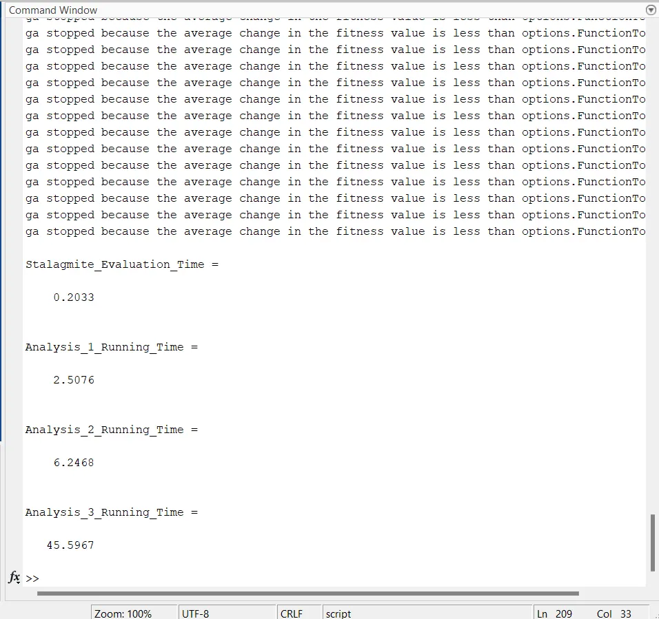
Fig 1
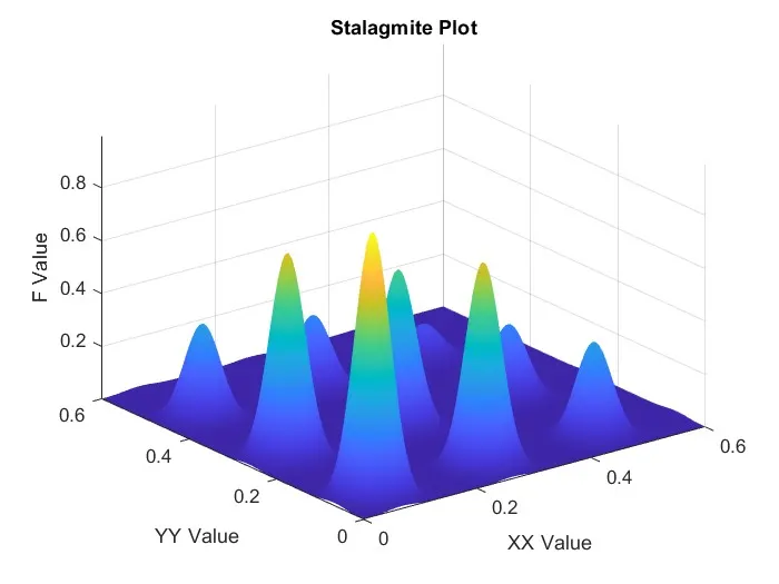
Fig 2
1. Case 1: Unbounded Inputs
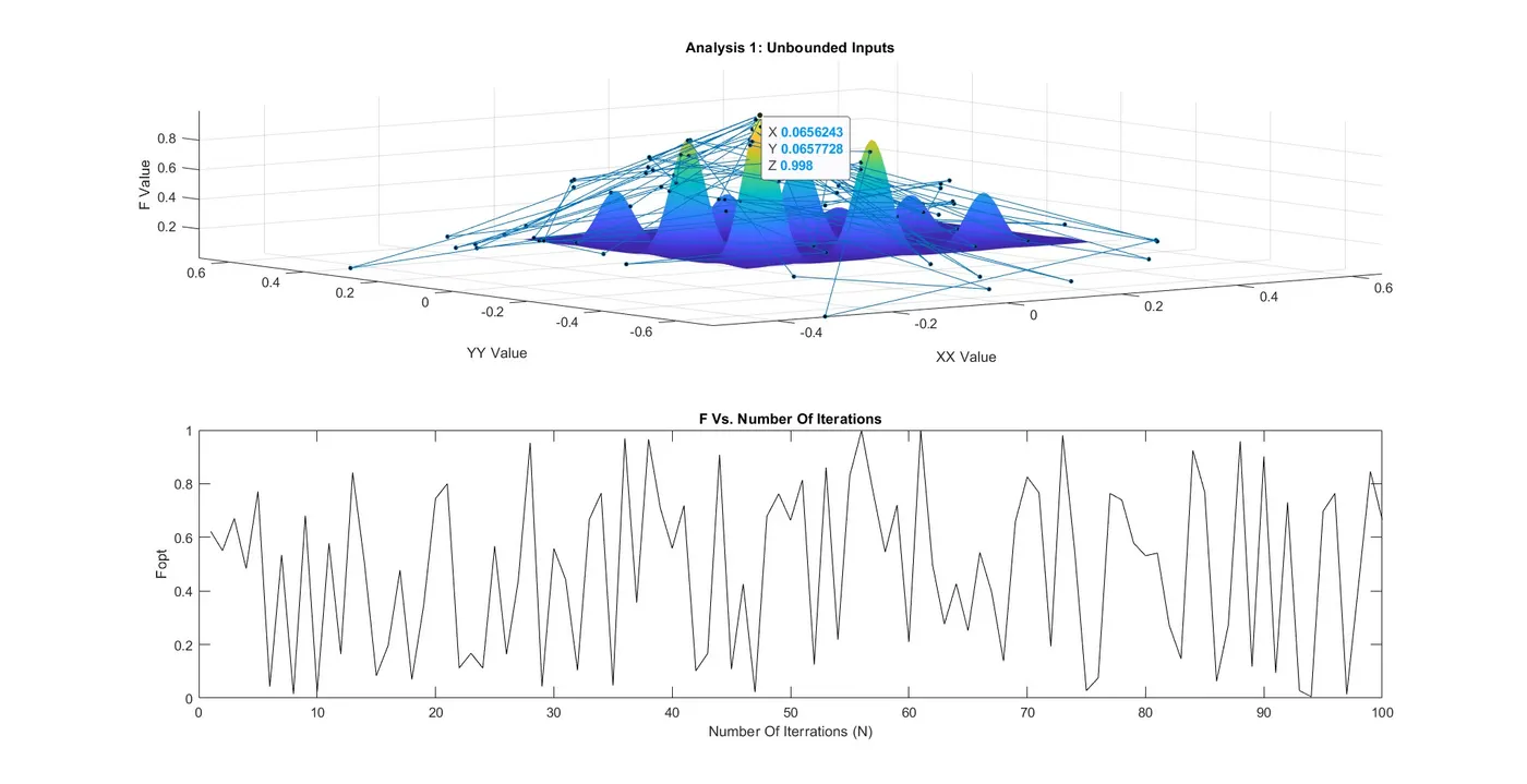
Fig 3
- Stimulation Time = 2.5076 Seconds
- Accuracy is very low. Because of unbounded inputs, we can see that the solutions spread outside the stalagmite area. The value of Fopt varies between is between 0 to 1.
- Stimulation time is much less.
2. Case 2: Bounded Inputs
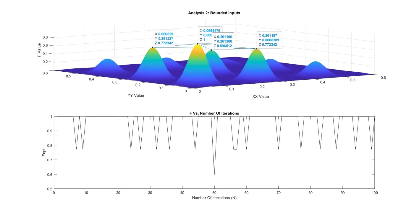
Fig 4
- Stimulation Time = 6.2428 Seconds
- Accuracy is high. The bounded inputs give only the four best outputs. The value of Fopt varies between 0.6 to 1.
- Stimulation time is high compared to the previous cases.
3. Case 3: Bounded Inputs With Increased Population.
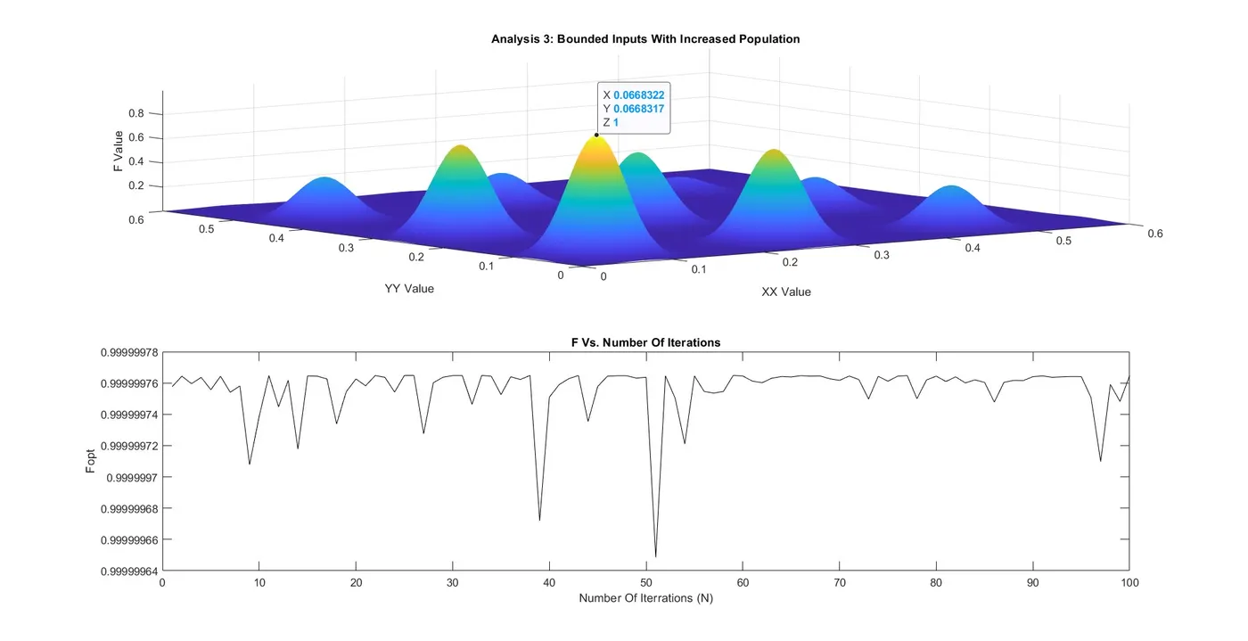
- Stimulation Time = 45.5967 Seconds
- Accuracy is very high. Gives only the best output. The value of Fopt varies from 0.9999 to 1.
- Stimulation time is very high compared to other cases.
Errors Faced During The Code Generation.
Hopefully, If we ignore the misspellings, there are no major errors present during the code developments