clear all % Code to optimise the Stalagmite function
close all
clc
<!-- [if mso]>
<![endif]-->
�fining the search space
x = linspace(0,0.6,150);
y = linspace(0,0.6,150);
n = 50; % no. of iterations
<!-- [if mso]>
<![endif]-->
[xx,yy] = meshgrid(x,y);
<!-- [if mso]>
<![endif]-->
% Evaluating stalagmite function
for i = 1:length(xx)
for j = 1:length(yy)
input_vector(1) = xx(i,j);
input_vector(2) = yy(i,j);
f(i,j) = stalagmite_func(input_vector);
end
end
<!-- [if mso]>
<![endif]-->
tic
�se 1 - Statistical Behaviour
for k = 1:n
[inputs1 , fopt1(k)] = ga(@stalagmite_func, 2);
xopt1(k) = inputs1(1);
yopt1(k) = inputs1(2);
end
study1_time = toc;
figure(1)
subplot(2,1,1)
hold on
surfc(xx,yy,-f)
shading interp
<!-- [if mso]>
<![endif]-->
plot3(xopt1,yopt1,-fopt1,'marker','o','markerfacecolor','r')
xlabel('X values')
ylabel('Y values')
title('Statistical Behaviour')
<!-- [if mso]>
<![endif]-->
figure(2)
plot(-fopt1)
xlabel('Iterations')
ylabel('fopt')
title('Statistical Behaviour')
<!-- [if mso]>
<![endif]-->
�se 2 - Statistical Behaviour - with upper and lower bound
for k = 1:n
[inputs2 , fopt2(k)] = ga(@stalagmite_func, 2,[],[],[],[],[0;0],[1;1]);
xopt2(k) = inputs2(1);
yopt2(k) = inputs2(2);
end
figure(3)
subplot(2,1,1)
hold on
surfc(xx,yy,-f)
shading interp
<!-- [if mso]>
<![endif]-->
plot3(xopt2,yopt2,-fopt2,'marker','o','markerfacecolor','r')
xlabel('X values')
ylabel('Y values')
title('Statistical Behaviour - with upper and lower bound')
<!-- [if mso]>
<![endif]-->
figure(4)
plot(-fopt2)
xlabel('Iterations')
ylabel('fopt')
title('Statistical Behaviour - with upper and lower bound')
<!-- [if mso]>
<![endif]-->
�se 3 - Statistical Behaviour - with increasing GA iterations
options = optimoptions('ga');
options = optimoptions(options,'populationsize',300);
<!-- [if mso]>
<![endif]-->
for k = 1:n
[inputs3 , fopt3(k)] = ga(@stalagmite_func, 2,[],[],[],[],[0;0],[1;1],[],[],options);
xopt3(k) = inputs3(1);
yopt3(k) = inputs3(2);
end
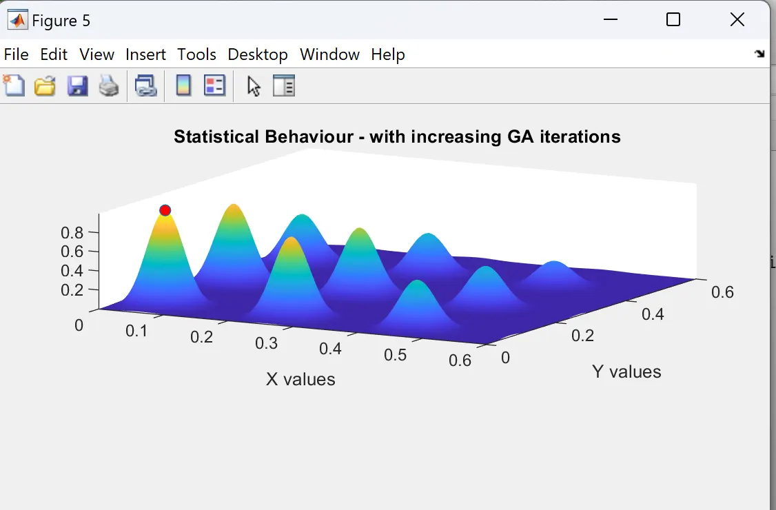
figure(5)
subplot(2,1,1)
hold on
surfc(xx,yy,-f)
shading interp
<!-- [if mso]>
<![endif]-->
plot3(xopt3,yopt3,-fopt3,'marker','o','markerfacecolor','r')
xlabel('X values')
ylabel('Y values')
title('Statistical Behaviour - with increasing GA iterations')
<!-- [if mso]>
<![endif]-->
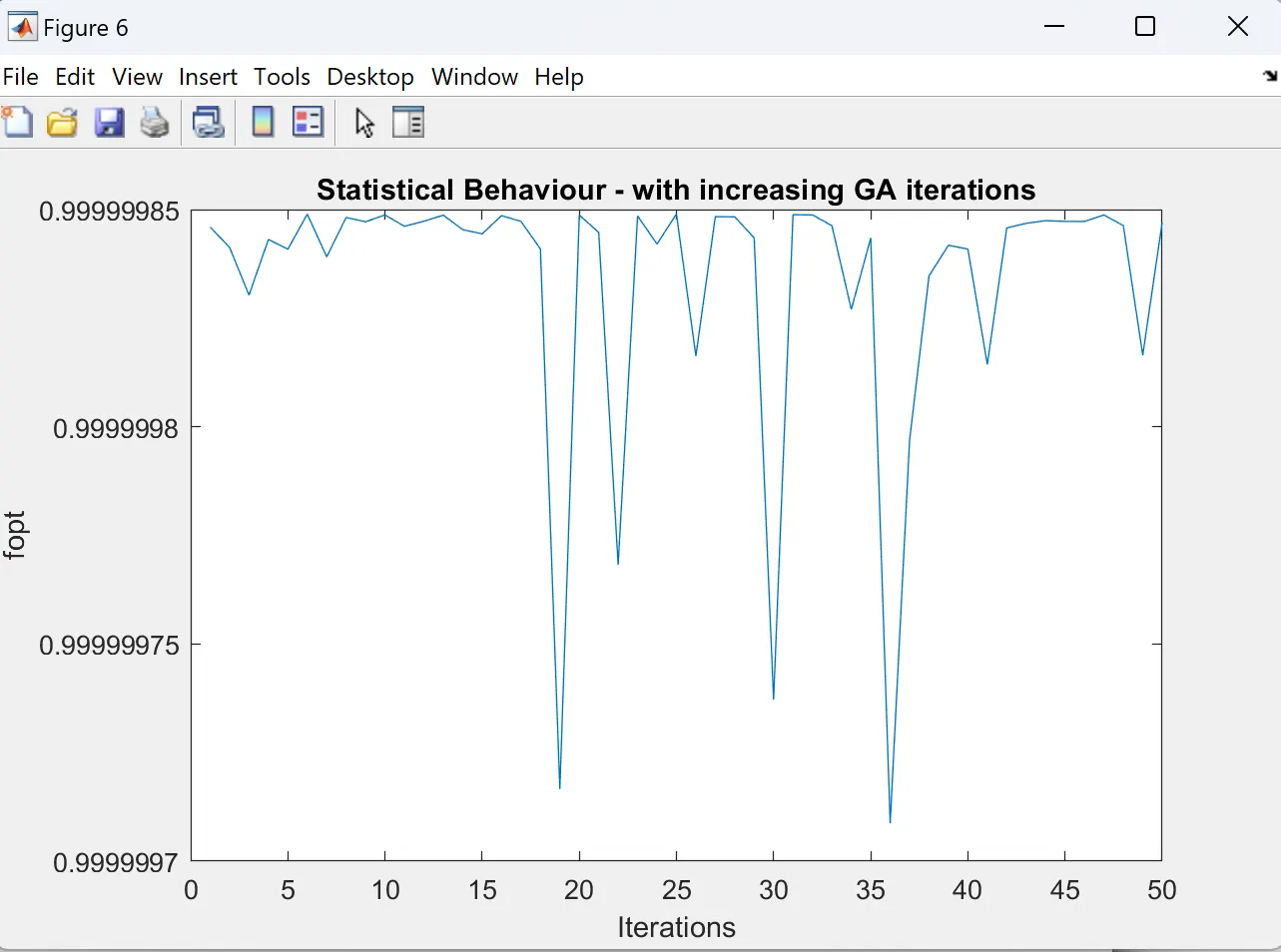
figure(6)
plot(-fopt3)
xlabel('Iterations')
ylabel('fopt')
title('Statistical Behaviour - with increasing GA iterations')
Program Code Explanation:-
Lines 1-3: Clear variables, close figures, and clear the console.
Lines 6-8: Define the x and y search space coordinates and the number of iterations (`n`).
Lines 12-15: Create a grid of x and y coordinates for the search space using `meshgrid`.
Lines 18-24: Iterate over each combination of x and y coordinates to evaluate the objective function and store results in matrix `f`.
Lines 27-33: Perform standard Genetic Algorithm (`ga`) optimization (`n` iterations) and store optimal inputs (`inputs1`), objective value (`fopt1`), and x/y values (`xopt1`, `yopt1`).
Lines 36-38: Create a figure to visualize the optimization process and convergence behavior.
Lines 41-49: Perform Genetic Algorithm optimization with upper and lower bounds (`[0;0]` to `[1;1]`) and store results.
Lines 52-56: Perform Genetic Algorithm optimization with increased population size (`populationsize` set to 300) and store results.
Lines 57-62: Create figures to visualize the optimization process and convergence behavior for the last scenario
Function Code:-
function [f] = stalagmite_func(input_vector)
x = input_vector(1);
y = input_vector(2);
<!-- [if mso]>
<![endif]-->
term1 = (sin((5.1*pi*x )+ 0.5))^6;
term2 = (sin((5.1*pi*y) + 0.5))^6;
term3 = exp(-4*log(2)*((x-0.0667)^2)/0.64);
term4 = exp(-4*log(2)*((y-0.0667)^2)/0.64);
<!-- [if mso]>
<![endif]-->
f = -(term1*term2*term3*term4);
end
Function Code Explanation :
Line 1: Function declaration with input argument 'input_vector' and output 'f'
Line 3-4: Extract the elements from 'input_vector' into variables 'x' and 'y'
Line 6-7: Calculate 'term1' and 'term2' involving sine functions and exponentiation
Line 9-10: Calculate 'term3' and 'term4' using exponential functions and algebraic expressions
Line 12: Calculate the final objective function value 'f' by multiplying the terms and negating the result.
Output:-
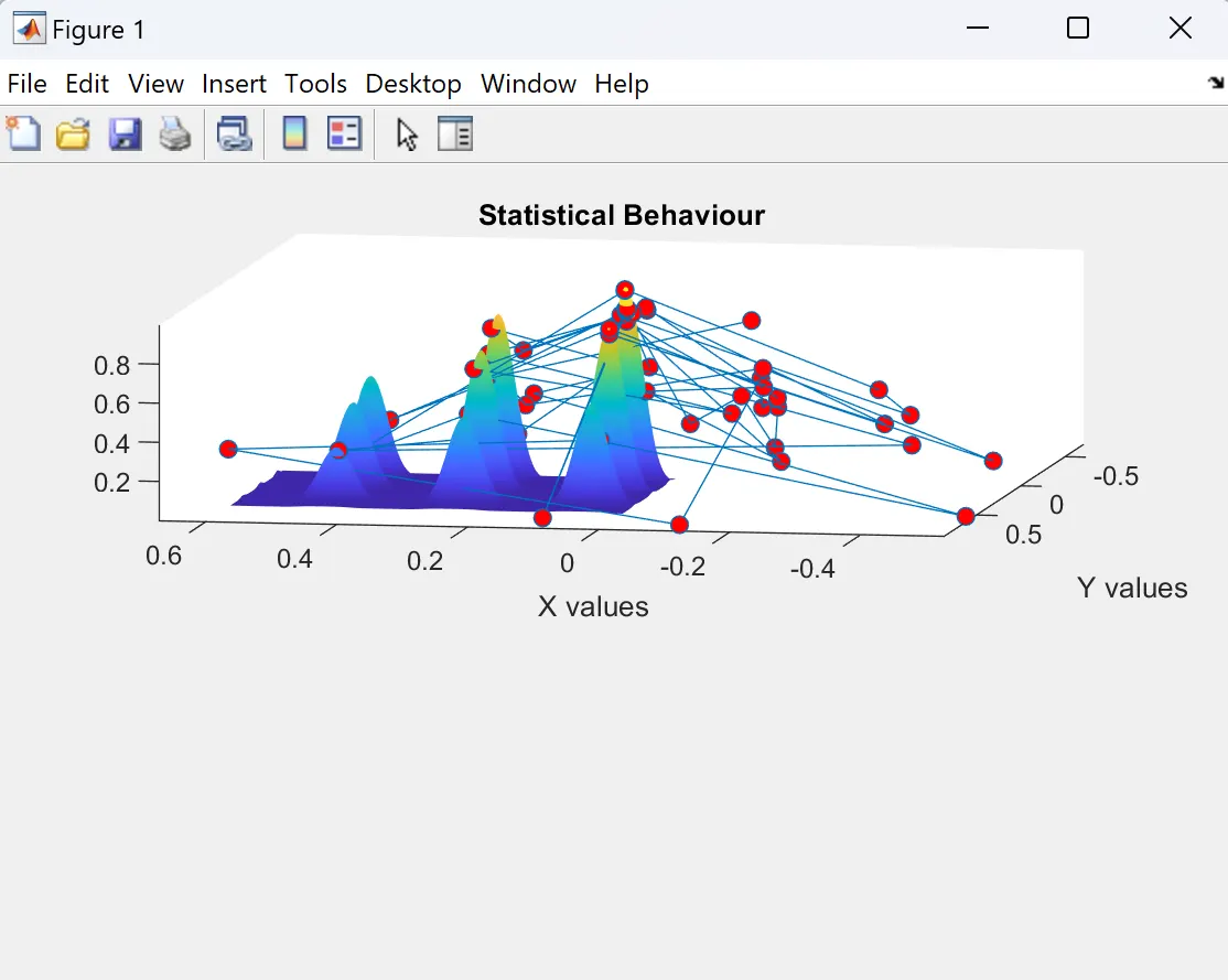
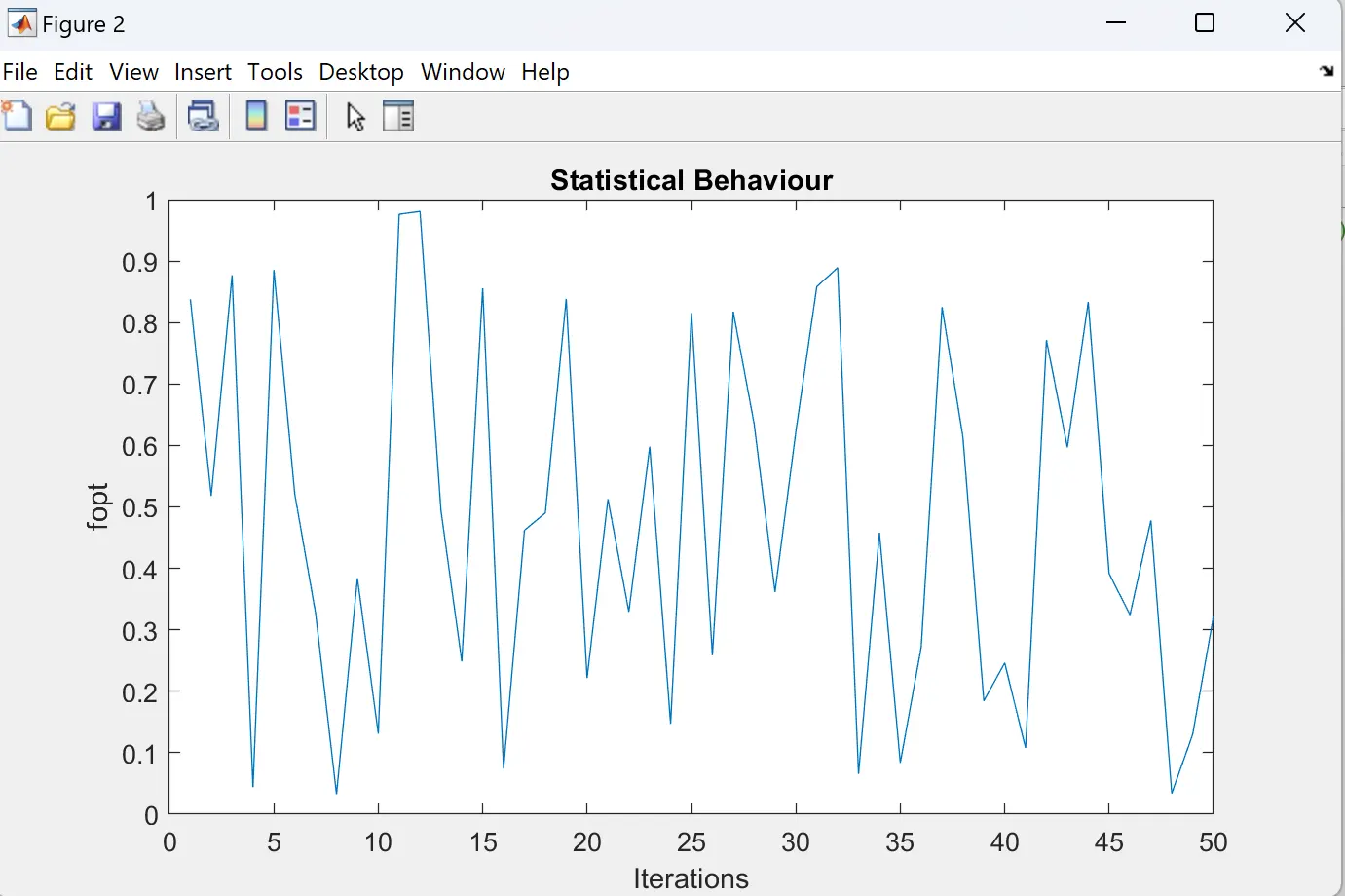
Case 1:- Statistical Bahaviour
Explanation:----
* The red dot shows no. of points or coordinates of x,y under consideration for each Iteration. Large no. of red dots shows values of coordinates of x,y.
* fopt vs iterations shows optimum value of function, fopt varies each time Iteration runs. It also shows large variations in fopt values of each iteration.
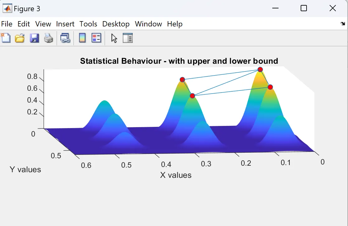
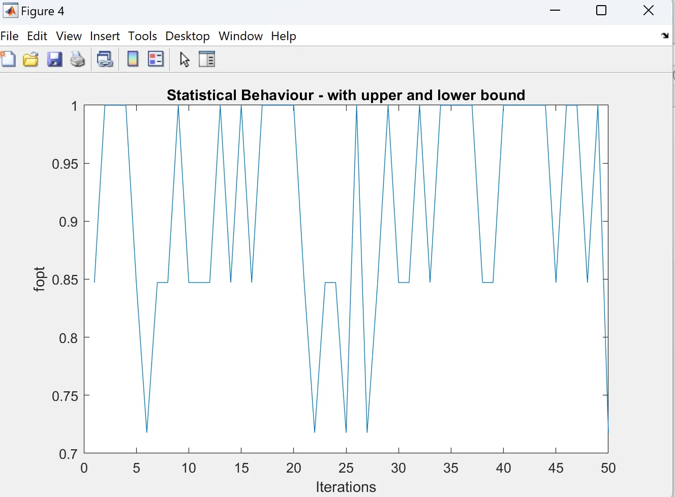
Case 2:-- Statistical Behaviour with Lower and Upper Bound
Explanation:--
* The above result shows coordinates of x,y are converging that of the previous case. No. of red dots are less showing values of x & y are not varying much as in the previous case. This is the result of providing
upper and lower bounds to the function.
* As bounds are provided, the value of function varies only in between prescribed limit i.e, 0 to 1. This reduces variation in function value with each iteration.
Case 3:--Statistical Behaviour with Increasing GA Iterations
Explanation:-----
* After providing upper-lower bounds and options, it seems that value of co-ordinates x,y coverges to only one value for each iteration. Values of x = 0.0668 & y = 0.0668.
* The Above graph shows that variations in values of a function are very low than that of other cases. The value of fopt comes out to be nearly 1.
-------
Genetic Algorithm:-
A genetic algorithm (GA) is a method for solving both constrained and unconstrained optimization problems based on a natural selection process that mimics biological evolution. The algorithm repeatedly modifies a population of individual solutions. At each step, the genetic algorithm randomly selects individuals from the current population and uses them as parents to produce the children for the next generation. Over successive generations, the population "evolves" toward an optimal solution.
You can apply the genetic algorithm to solve problems that are not well suited for standard optimization algorithms, including problems in which the objective function is discontinuous, nondifferentiable, stochastic, or highly nonlinear.
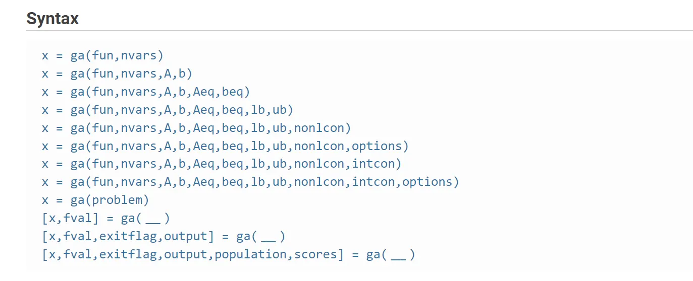
Syntax for 'ga' in Matlab:-
The ‘ga’ syntax in Matlab is used to find the minimum of a function using a genetic algorithm. There are several ways to define the ‘ga’ function depending on the problem being solved. The syntax used for this study is shown below.
Error:- No errors found while excecuting the code.
References:-
https://www.mathworks.com/discovery/genetic-algorithm.html
https://www.mathworks.com/help/gads/ga.html
https://skill-lync.com/student-projects/Optimization-of-Stalagmite-function-using-Genetic-Algorithm-in-MATLAB-53317