Week 5 - Genetic Algorithm
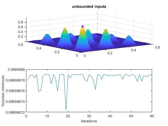
AIM: To write a code in MATLAB to optimize the stalagmite function and find the global maxima of the function. To explain the concept of genetic algorithm and also the syntax for ga in MATLAB. To plot the graphs for all 3 studies and for F maximum vs no. of iterations.
Theory: Stalagmites are rocks that rise from the floor of a cave due to the accumulation of materials from drops from the ceiling. The shape of these stalagmites are the basis for calling these programs as "STALAGMITES".
Genetic Algorithm is a method based on natural selection, the basis of biological evolution, for addressing both limited and unconstained optimization problems. The population size of distinct solution is always changing thanks to evolutionary algorithm.
Phases of Genetic Algorithm:
- Initialization of Population: Each gene stands for a parameter in the response. The chromosome is this set of variables that makes up the solution.
- Fitness Function: Out of the available chromosomes, we must choose the finest ones to create offspring, hence each chromosome is assigned a fitness value.
- Selection: Finding the area where getting the greatest answer is more likely the major objective of theis phase.
- Reproduction: Generation of offsprings happen by two ways:
- Crossover: Crossover is the most vital stage in the Genetic Algorithm. During a crossover a random point is selected while mating a pairof parents, to generate offspring.
- Mutation: Some of the newly produced offsprings may be subjected to low probability mutation. This suggests that some bits of the chromosome can be switched around. Mutation occurs to maintain population variety and to prevent premature convergence.
- Convergence (When to stop): Following are the conditions which determine when to stop:
- when a predetermined number of generations have passed and there is no improvement in the quality of the answer.
- when a fixed number of generations or years have passed.
- until a workable resolution is found.
Syntax for Genetic Algorithm:
[x,fval,exitflag,output,population,scores]=ga(func,nvars,A,b,Aeq,beq,lb,ub,nonIcon,IntCon,options)
where,
- x - optimum solution
- exitflag - reason Genetic Algorithm stopped
- output - information about optimization process
- population - final population
- scores - final scores
- func - fitness function
- nvars - number of variables
- A,b - linear contraints
- Aeq,beq - linear equality contraints
- lb,ub - lower and upper bounds (limits)
- nonIcon - use of non-linear constraints
- IntCon - to get solution in integer
- options - to set the population size with non-default options
Function Code:
function [f] = stalagmite(input_vector)
x = input_vector(1);
y = input_vector(2);
f1x = (sin(5.1*pi*x + 0.5))^6;
f1y = (sin(5.1*pi*y + 0.5))^6;
f2x = exp((-2.7726)*(x-(0.0667))^2/0.46);
f2y = exp((-2.7726)*(y-(0.0667))^2/0.46);

f = -(f1x*f1y*f2x*f2y);
endExplanation:
- function to perform the task of stalagmite function
- initialize first column
- initialize second column
- initialize terms according to equation
- calculation the value according to the stalagmite function
Main Code:
clear all
close all
clc

%Defining our search space
x = linspace(0,0.6,150);
y = linspace(0,0.6,150);
num_case = 60;

%creating a 2Dimensional mesh
[xx yy] = meshgrid(x,y);

%Evaluating the stalagmite function

for i = 1:length(xx)
    for j = 1:length(yy)
        input_vector(1)=xx(i,j);
        input_vector(2)=yy(i,j);
        f(i,j) = stalagmite(input_vector);
    end
end

tic
for k = 1:num_case;
    [inp, fval(k)] = ga(@stalagmite,2);
    x_1(k) = inp(1);
    y_1(k) = inp(2);
end
study1_time = toc

figure (1)
hold on
grid on
surfc(xx,yy,-f)
shading interp
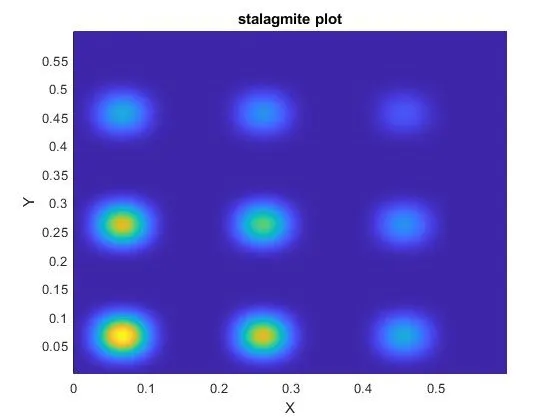
title('stalagmite plot')
xlabel('X')
ylabel('Y')

figure(2)
subplot(2,1,1)
surfc(xx,yy,-f)
shading interp
hold on
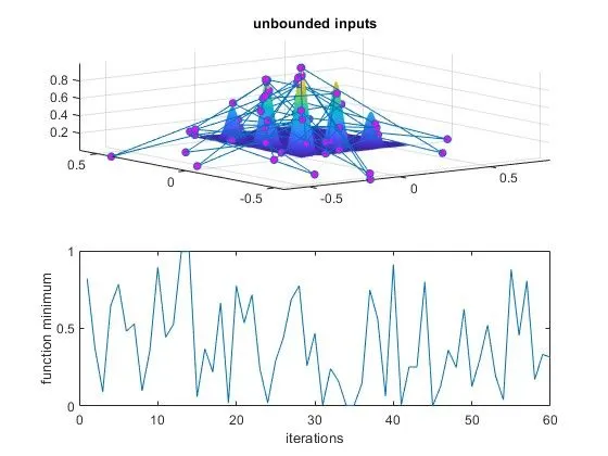
plot3(x_1,y_1,-fval,'marker','o','MarkerSize',5,'MarkerFaceColor','m')
title('unbounded inputs')
subplot(2,1,2)
plot(-fval)
xlabel('iterations')
ylabel('function minimum')


% 2nd case study statistical behaviour
tic
for s = 1:num_case;
    [input,fval(s)]= ga(@stalagmite,2,[],[],[],[],[0,0],[0.6,0.6]);
    x_2(s)= input(1);
    y_2(s)= input(2);

end
study2_time = toc;
figure(3)
subplot(2,1,1)
surfc(xx,yy,-f)
shading interp
hold on
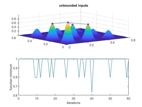
plot3(x_2,y_2,-fval,'marker','o','MarkerSize',5,'MarkerFaceColor','m')
title('unbounded inputs')
subplot(2,1,2)
plot(-fval)
xlabel('iterations')
ylabel('function minimum')

% 3rd case study increasing ga iterations
options = optimoptions('ga');
options = optimoptions(options,'PopulationSize',500);

tic
for m = 1:num_case;
    [input,fval(m)]= ga(@stalagmite,2,[],[],[],[],[0,0],[0.6,0.6],[],[],options);
    x_3(m)= input(1);
    y_3(m)= input(2);

end
study3_time = toc
figure(4)
subplot(2,1,1)
surfc(xx,yy,-f)
shading interp
hold on
plot3(x_3,y_3,-fval,'marker','o','MarkerSize',5,'MarkerFaceColor','m')
title('unbounded inputs')
subplot(2,1,2)
plot(-fval)
xlabel('iterations')
ylabel('function minimum')Explanation:
- clear all the workspace variables
- close all the output window
- clear the command window
- linspace is used to generate 150 values between 0 and 0.6
- create a dimensional array
- execution of the statements in loop till length(xx)
- execution of the statements in loop till length(yy)
- initialize array rows and column
- call the stalgamite function to get the value by passing input vector
- terminate the for loop
- generate a surface plot
Output:
Stalagmite Function:
Case Study 1:
Case Study 2:
Case Study 3:
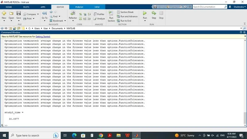
Study Time: