Week 3 - Solving second order ODEs

AIM:

To write a program in MATLAB to simulate the transient behaviour of a simple pendulum and to create an animation of its motion.

THEORY:

A simple pendulum consists of a mass m, suspended by a length l, from a fixed point having a damping coefficient b.

The ordinary differential equation for the motion of the simple pendulum is

`(d^2theta)/(dt^2)+(b/m)(d theta)/(dt)+(g/l)sintheta=0`

where,

b = damping coefficient

m = mass

g = acceleration due to gravity

l = length of the pendulum

To solve the second order ODE, we split the equation into first order ODE.

`(d^2theta)/(dt^2)+(b/m)(d theta)/(dt)+(g/l)sintheta=0`

let, `theta=theta1`

then, `(d theta)/(dt)=(d theta1)/(dt)=theta2`

`(d theta2)/(dt)+(b/m)theta2+(g/l) sintheta1=0`

`(d theta2)/(dt)= -(b/m)theta2-(g/l)sintheta1`

Program:

clear all
close all
clc
%FIXED PARAMETERS - (1)
%DAMPING COEFFICIENT
b=0.05;
%ACCELERATION DUE TO GRAVITY
g=9.81;
%MASS
m=1;
%LENGTH
l=1;
%INITIAL CONDITION - (2)
theta_0=[0;3];
%TIME POINTS
t_span=linspace(0,20,500);
%SOLVING ODE - (3)
[t,results]=ode45(@(t,theta)ode_funs(t,theta,b,g,l,m),t_span,theta_0);
%PLOTTING - (4)
figure(1)
plot(t,results(:,1))
hold on
plot(t,results(:,2))
xlabel('TIME')
ylabel('VELOCITY(Red) & DISPLACEMENT(Blue)')
%ANIMATION - (5)
ct=1;
for i=1:length(results(:,1))
x0=0;
y0=0;
x1=l*sin(results(i,1)+pi);
y1=l*cos(results(i,1)+pi);
figure(2)
plot([x0 x1],[y0 y1],'-o','MarkerSize',10,'MarkerFaceColor','r','MarkerEdgeColor','r','LineWidth',4)
axis([-2 2 -2 2])
hold on
plot([-1 1],[0,0],'LineWidth',5,'Color','[0 0.3 0]')
pause(0.01)
M(ct)=getframe(gcf);
hold off
ct-ct+1;
end
%MOVIE & FILE - (6)
movie(M)
videofile=VideoWriter('Pendulum_Challenge.avi','Uncompressed AVI');
open(videofile)
writeVideo(videofile,M)
close(videofile)

Function Program:

%ODE FUNCTION
function dtheta_dt=ode_funs(t,theta,b,g,l,m)
theta1=theta(1);
theta2=theta(2);
dtheta1_dt=theta2;
dtheta2_dt=-(b/m)*theta2-(g/l)*sin(theta1);
dtheta_dt=[dtheta1_dt;dtheta2_dt];
end

Explanation:

1. The constants, damping coefficient, length of the pendulum, acceleation due to gravity and mass are entered.

2. `theta` is entered as a column matrix and timespan is entered through a linspace command.

3. A solver ode45 is used, where it gets the values such as time span, theta_0 and define it into the user defined functions and returns into [t,results].

4. Then the results are plotted to get the transient behaviour of the pendulum motion.

5. the 'for' loop is used to plot the displacement of the pendulum at various angles of `theta`. A counter variable 'ct' is used to get every frame of displacement usingg 'getframe' command.

6. Movie command is used to create a video file.

OUTPUT:

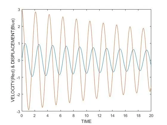
Errors:

There is an error in the program in the video file part which is not allowing the complete animation to convert to a video.