Week 5 - Genetic Algorithm
Aim:
To write a code for optimising the stalagmite function and also to find the global maxima of the stalagamite function.
What is genetic algorithm and its syntax in Matlab?
Genetic Algorithm (GA) is a search-based optimization technique inspired by the process of natural selection and genetics. It is a method of solving optimization problems that involve searching for the optimal solution in a large search space by imitating the natural process of evolution.
The basic idea behind GA is to represent a potential solution to the problem as a string of binary or real values, which is called a chromosome. The algorithm then applies genetic operators such as selection, crossover, and mutation to create a new population of chromosomes. The fitness of each chromosome in the population is evaluated, and the ones that are most fit are selected for the next generation. This process is repeated until a satisfactory solution is found.
In MATLAB, GA is implemented using the 'ga' function. The syntax of the 'ga' function is as follows:
[x,fval] = ga(fun,nvars)
[x,fval] = ga(fun,nvars,A,b)
[x,fval] = ga(fun,nvars,A,b,Aeq,beq)
[x,fval] = ga(fun,nvars,A,b,Aeq,beq,LB,UB)
[x,fval,exitflag,output,population,scores] = ga(___)
where
- 'fun' - fitness function that is to be minimized or maximized.
- 'nvars' - number of variables in the optimization problem.
- 'A' and 'b' - linear inequality constraints.
- 'Aeq' and 'beq' - linear equality constraints.
- 'LB' and 'UB' - lower and upper bounds of the variables.
- 'x' - solution vector that minimizes the fitness function 'fun'.
- 'fval' - value of the fitness function at the solution 'x'.
- 'exitflag' - integer code that indicates the reason for the termination of the algorithm.
- 'output'- structure containing information about the optimization process.
- 'population' and 'scores' - final population of chromosomes and their corresponding fitness values.
Matlab code:
clear all
close all
clc
% Defining our search space
x=linspace(0,0.6,150);
y=linspace(0,0.6,150);
num_cases=50;

% creating 2D mesh
[xx, yy]=meshgrid(x,y);

%Evaluating the stalagmite function
for i=1:length(xx)
    for j=1:length(yy)
        input_vector(1)=xx(i,j);
        input_vector(2)=yy(i,j);
        f(i,j)=stalagmite(input_vector);
    end
end

% study 1- statistical behavior
for i=1:num_cases
    [inputs,fopt(i)]=ga(@stalagmite,2);
    xopt(i)=inputs(1); % optimisation inputs
    yopt(i)=inputs(2);
end
fopt=-fopt; % negative sign for finding global maxima
f=-f;
figure(1)
subplot(2,1,1)
hold on
surfc(x,y,f)
shading interp
plot3(xopt,yopt,fopt,'marker','o','markersize',5,'markerfacecolor','r')
title('unbounded inputs')
subplot(2,1,2)
plot(fopt)
xlabel('Iterations')
ylabel('Function maximum')

 tic
% study 2 - statistical behaviour with upper and lower bounds
for i=1:num_cases
    [inputs,fopt(i)]=ga(@stalagmite,2,[],[],[],[],[0;0],[1;1]);
    xopt(i)=inputs(1);
    yopt(i)=inputs(2);
end
fopt=-fopt;
f=-f;
 toc
figure(2)
subplot(2,1,1)
hold on
surfc(x,y,f)
shading interp
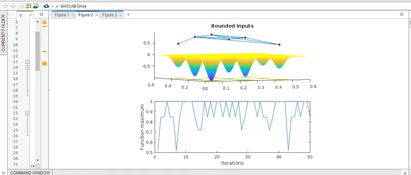
plot3(xopt,yopt,fopt,'marker','o','markersize',5,'markerfacecolor','r')
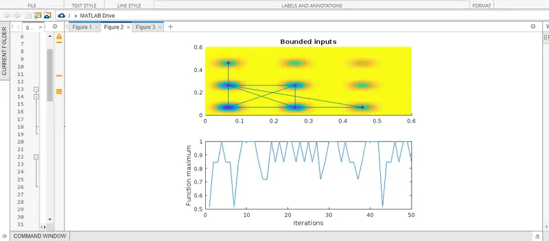
title('Bounded inputs')
subplot(2,1,2)
plot(fopt)
xlabel('Iterations')
ylabel('Function maximum')

%study 3 Incresing GA iterations
options= optimoptions('ga');
options=optimoptions(options,'PopulationSize',150);

 tic
for i=1:num_cases
    [inputs,fopt(i)]=ga(@stalagmite,2,[],[],[],[],[0;0],[1;1],[],[],options);
    xopt(i)=inputs(1);
    yopt(i)=inputs(2);
end
fopt=-fopt;
f=-f;
 toc
figure(3)
subplot(2,1,1)
hold on
surfc(x,y,f)
shading interp
plot3(xopt,yopt,fopt,'marker','o','markersize',5,'markerfacecolor','r')
title('Bounded inputs with incresing population')
subplot(2,1,2)
plot(fopt)
xlabel('Iterations')
ylabel('Function maximum')
Code for stalagmite function:
function f=stalagmite(input)
x=input(1);
y=input(2);
f1x=(sin(((5.1*pi).*x)+0.5)).^6;
f1y=(sin(((5.1*pi).*y)+0.5)).^6;
f2x=exp((((x-0.0667).^2).*(-4*log(2)))./0.64);
f2y=exp((((y-0.0667).^2).*(-4*log(2)))./0.64);
f=-f1x*f1y*f2x*f2y;
end
Results:
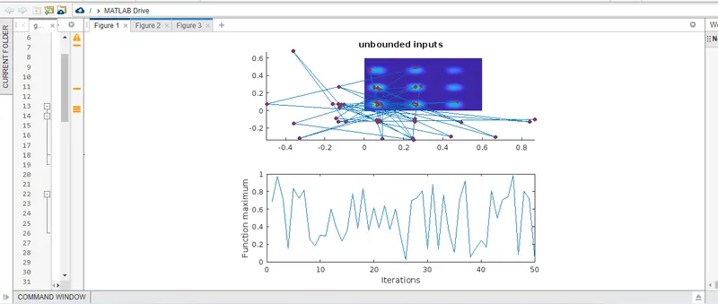
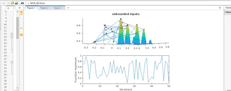
1D and 3D graphs for 'unbounded inputs' are shown below. This graph varies from 0 to 1 in the Y-axis and 0 to 50 in the X-axis. Between 1 to 10 and 45 to 50 iterations, the global maxima occur.
1D and 3D graphs for 'bounded inputs' are shown below. For same 50 iterations with bounded inputs, we can see the graph bit clear.
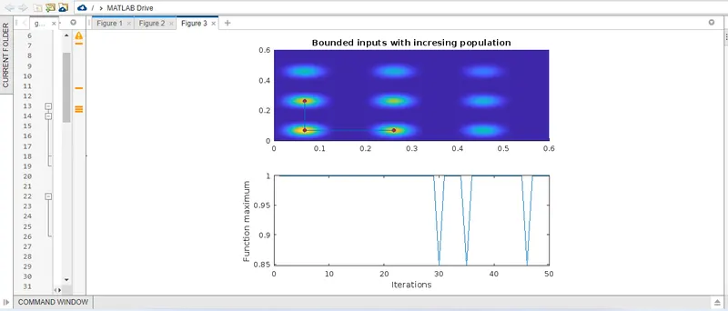
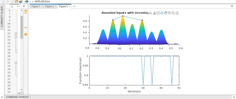
1D and 3D graphs for bounded inputs with modified population are given below. Here, we can see the less number of global maxima points.