Week 3.5 - Deriving 4th order approximation of a 2nd order derivative using Taylor Table method
Aim:
To derive central, skewed right sided and skewed left sided difference schemes and to prove these skewed schemes are fourth order accurate.
What is Taylor series?
Taylor table is also known as Taylor series, is a representation of a function as an infinite sum of terms that are calculated from the function’s derivatives at a specific point. This gives an approximation of the function value near that point.
1.Central difference scheme:
The central difference scheme utilizes the values of the function at two neighbouring points to estimate the derivative.
For central difference /symmetric schemes, the order of accuracy P = Number of nodes in the stencil N – order of derivative Q + 1.
So, N = P + Q -1, N = 4+2 -1 = 5
---------*----------*----------*----------*----------*---------
(i-2) (i-1) (i) (i+1) (i+2)
Second order derivative for 4th order approximation for central differencing scheme is
d^2/dx^2 = a f(i-2) +b f(i-1) +c f(i) + d f(i+1) + e f(i+2)
|
Stencil |
f(i) |
dx f’(i) |
(dx^2) f’’(i) |
(dx^3) f’’’(i) |
(dx^4) f’’’’(i) |
|
a f(i-2) |
a |
-2a |
2a |
-8a/6 |
16a/24 |
|
b f(i-1) |
b |
-b |
b/2 |
-b/6 |
b/24 |
|
c f(i) |
c |
0 |
0 |
0 |
0 |
|
d f(i+1) |
d |
d |
d/2 |
d/6 |
d/24 |
|
e f(i+2) |
e |
2e |
2e |
8e/6 |
16e/24 |
|
Sum |
0 |
0 |
1 |
0 |
0 |
2.Skewed right sided scheme:
The skewed right sided scheme utilizes the values of the function at points towards its right to estimate the derivative.
For skewed right sided scheme, the order of accuracy P = Number of nodes in the stencil N – order of derivative Q.
So, N = P + Q, N = 4+2 = 6
---------*----------*----------*----------*----------*-----------*--------
(i) (i+1) (i+2) (i+3) (i+4) (i+5)
Second order derivative for 4th order approximation for skewed right sided scheme is
d^2/dx^2 = a f(i) +b f(i+1) +c f(i+2) + d f(i+3) + e f(i+4) + g f(i+5)
|
Stencil |
f(i) |
dx f’(i) |
(dx^2) f’’(i) |
(dx^3) f’’’(i) |
(dx^4) f’’’’(i) |
(dx^5) f’’’’’(i) |
|
a f(i) |
a |
0 |
0 |
0 |
0 |
0 |
|
b f(i+1) |
b |
b |
b/2 |
b/6 |
b/24 |
b/120 |
|
c f(i+2) |
c |
2c |
4c/2 |
8c/6 |
16c/24 |
32c/120 |
|
d f(i+3) |
d |
3d |
9d/2 |
27d/6 |
81d/24 |
243d/120 |
|
e f(i+4) |
e |
4e |
16e/2 |
64e/6 |
256e/24 |
1024e/120 |
|
g f(i+5) |
g |
5g |
25g/2 |
125g/6 |
625g/24 |
3125g/120 |
|
Sum |
0 |
0 |
1 |
0 |
0 |
0 |
3.Skewed left sided differences:
The skewed leftt sided scheme utilizes the values of the function at points towards its left to estimate the derivative.
For skewed left sided scheme, the order of accuracy P = Number of nodes in the stencil N – order of derivative Q.
So, N = P + Q, N = 4+2 = 6
---------*----------*----------*----------*----------*-----------*--------
(i) (i-1) (i-2) (i-3) (i-4) (i-5)
Second order derivative for 4th order approximation for skewed left sided scheme is
d^2/dx^2 = a f(i) +b f(i-1) +c f(i-2) + d f(i-3) + e f(i-4) + g f(i-5)
|
Stencil |
f(i) |
dx f’(i) |
(dx^2) f’’(i) |
(dx^3) f’’’(i) |
(dx^4) f’’’’(i) |
(dx^5) f’’’’’(i) |
|
a f(i) |
a |
0 |
0 |
0 |
0 |
0 |
|
b f(i-1) |
b |
-b |
b/2 |
-b/6 |
b/24 |
-b/120 |
|
c f(i-2) |
c |
-2c |
4c/2 |
-8c/6 |
16c/24 |
-32c/120 |
|
d f(i-3) |
d |
-3d |
9d/2 |
-27d/6 |
81d/24 |
-243d/120 |
|
e f(i-4) |
e |
-4e |
16e/2 |
-64e/6 |
256e/24 |
-1024e/120 |
|
g f(i-5) |
g |
-5g |
25g/2 |
-125g/6 |
625g/24 |
-3125g/120 |
|
Sum |
0 |
0 |
1 |
0 |
0 |
0 |
MATLAB code:
MATLAB code for analytical function of fourth order approximation is given below,
Analytical derivative = exp(x)*cos(x)
= -2*sin(x)*exp(x)
clear all
close all
clc
%inputs
x=pi/3;
dx=linspace(pi/4,pi/4000,100);

%for loop for the range of range of dx

for i = 1:length(dx)
    %formulas for errors
    central_diff_error(i)=central_diff(x,dx(i));
    skewed_right_error(i)=skewed_right_diff(x,dx(i));
    skewed_left_error(i)=skewed_left_diff(x,dx(i));
end

%plotting the graphs
figure(1)
%loglog command is used for enlarged graphs
loglog(dx,central_diff_error,'k','Marker','o')
hold on
loglog(dx,skewed_right_error,'b','Marker','*')
hold on
loglog(dx,skewed_left_error,'g','Marker','.')
%giving labels, title, legend for understanding the graph
xlabel('dx')
ylabel('Errors')
title('Range of dx vs Errors')
legend('central difference','skewed right sided diff','skewed left sided diff')


%function for central difference
function out = central_diff(x,dx)
j=[1 1 1 1 1;-2 -1 0 1 2;2 1/2 0 1/2 2;-8/6 -1/6 0 1/6 8/6;16/24 1/24 0 1/24 16/24];
k=[0;0;1;0;0];
l=inv(j)*k
%analytical_derivative=-2*sin(x)*exp(x);
analytical_derivative=-2*sin(x)*exp(x);
central_diff_approxi=(l(1)*exp(x-2*dx)*cos(x-2*dx)+l(2)*exp(x-dx)*cos(x-dx)+l(3)*exp(x)*cos(x)+l(4)*exp(x+dx)*cos(x+dx)+l(5)*exp(x+2*dx)*cos(x+2*dx))/((dx)^2);
out=abs(central_diff_approxi-analytical_derivative);
end

%function for right sided difference
function out = skewed_right_diff(x,dx)
t=[1 1 1 1 1 1;0 1 2 3 4 5;0 1/2 4/2 9/2 16/2 25/2;0 1/6 8/6 27/6 64/6 125/6;0 1/24 16/24 81/24 256/24 625/24;0 1/120 32/120 243/120 1024/120 3125/120];
u=[0;0;1;0;0;0];
v=inv(t)*u

analytical_derivative=-2*sin(x)*exp(x);
skewed_right_diff_approxi=(v(1)*exp(x)*cos(x)+v(2)*exp(x+dx)*cos(x+dx)+v(3)*exp(x+2*dx)*cos(x+2*dx)+v(4)*exp(x+3*dx)*cos(x+3*dx)+v(5)*exp(x+4*dx)*cos(x+4*dx)+v(6)*exp(x+5*dx)*cos(x+5*dx))/((dx)^2);
out=abs(skewed_right_diff_approxi-analytical_derivative);
end

%function for left sided difference
function out = skewed_left_diff(x,dx)
p=[1 1 1 1 1 1;0 -1 -2 -3 -4 -5;0 1/2 4/2 9/2 16/2 25/2;0 -1/6 -8/6 -27/6 -64/6 -125/6;0 1/24 16/24 81/24 256/24 625/24;0 -1/120 -32/120 -243/120 -1024/120 -3125/120];
q=[0;0;1;0;0;0];
r=inv(p)*q

analytical_derivative=-2*sin(x)*exp(x);
skewed_left_diff_approxi=(r(1)*exp(x)*cos(x)+r(2)*exp(x-dx)*cos(x-dx)+r(3)*exp(x-2*dx)*cos(x-2*dx)+r(4)*exp(x-3*dx)*cos(x-3*dx)+r(5)*exp(x-4*dx)*cos(x-4*dx)+r(6)*exp(x-5*dx)*cos(x-5*dx))/((dx)^2);
out=abs(skewed_left_diff_approxi-analytical_derivative);
end
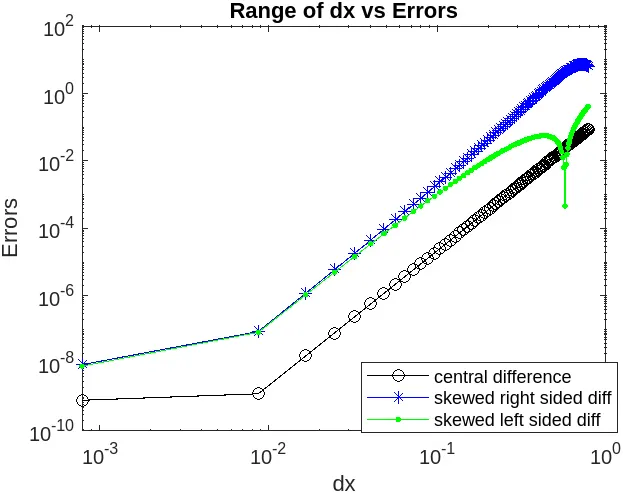
Graph:
Explanation:
1. Skewed right sided difference scheme shows maximum when compared to other two errors.
2. Skewed left sided error almost equal to skewed right sided error till 10^-1, after that it becomes unstable and drop down below the central difference scheme.
3. Central difference scheme shows minimum error when compared to other two errors. For good accuracy, central difference scheme is preferrable.
We can see that the slope values for all the three schemes are similar.
Why a skewed scheme is useful? What can a skewed scheme do that a CD scheme cannot?
-
One-sided Information: A skewed scheme uses information from only one side of a point to approximate the derivative. In contrast, the central difference scheme uses data from both sides of the point. This difference in information can be advantageous when the function has an asymmetric behavior or when the available data is limited on one side.
-
Boundary Conditions: Skewed schemes are particularly useful when dealing with boundary points or near-boundary points where there is no data available on one side. For instance, if we want to approximate the derivative at the rightmost point of a dataset, a right-sided difference scheme can provide a suitable approximation by utilizing only the available data points to the right.
-
Accuracy and Stability: Skewed schemes may have different accuracy and stability characteristics compared to the central difference scheme. While central difference schemes tend to provide more accurate approximations for smooth functions, skewed schemes can be more suitable for functions with specific characteristics or when dealing with limited data on one side.
Central difference scheme: A function with symmetric behavior utilizes CDS.
Skewed scheme : A function with asymmetric behavior utilizes skewed schemes.