Week 5.1 - Mid term project - Solving the steady and unsteady 2D heat conduction problem

Introduction:

In this mid-term project, we analyse 2D heat conduction by using different iterative methods. Also, we are comparing the convergence rates of different iterative methods to understand the numerical characteristics. We will implement iterative methods such as Jacobi, Gauss-Seidel, and Successive over relaxation for solving implicit equations.

Aim:

To solve 2D heat conduction equations for both steady and unsteady state using iterative methods. To compare the convergence rates of different methods for understanding the numerical characteristics.

Objectives:

1. Solve steady state equations using three different iterative methods

2. Analyse the convergence rates and simulation time.

3. Solve unsteady state using implicit and explicit schemes. For implicit schemes, use three iterative methods.

4. Compare the convergence rates and then compare overall convergence rates and simulation time for steady and unsteady state.

What is Implicit and Explicit schemes?

Implicit schemes:

Implicit scheme is a computational method used to solve differential equations such as 2D heat conduction equation, in which the values at the future time steps are determined using equation involving current and future values.

By using an implicit scheme, the transient behaviour of the heat conduction equation can be accurately captured, even for larger timesteps.

Explicit schemes:

Explicit schemes is also a computational method used to differential equation using solely the current values. It updates the temperature distribution at each time step by using current values. To satisfy the CFL stability criteria, time step must be small enough.

Steady state 2D heat conduction equation:

Distribution of temperature in a two dimensional domain. Steady state refers to the state where the temperature distribution remains constant over time. The equation is given by

`nabla^2T=0`

where, `nabla^2T=( partial ^2T)/(partialx^2)+( partial ^2T)/(partialy^2)`

This equation resembles elliptic nature, so we are using central differencing scheme for the above equation. we get,

`(T_(i+1,j)-2T_(i,j)+T_(i-1,j))^n/(trianglex^2)+(T_(i,j+1)-2T_(i,j)+T_(i,j-1))^n/(triangley^2)`

By solving,

`T_(i,j)=(1/k)*(T_(i-1,j)+T_(i+1,j))/(trianglex^2)+(T_(i,j+1)+T_(i,j-1))/(triangley^2)`

where `k=2*(trianglex^2+triangley^2)/(trianglex^2*triangley^2)`

For Jacobi, the above equation becomes,

`T_(i,j)^(n+1)=(1/k)*((T_(i-1,j)+T_(i+1,j))/(trianglex^2)+(T_(i,j+1)+T_(i,j-1))/(triangley^2))^n`

For Gauss-Seidel,

`T_(i,j)^(n+1)=(1/k)*((T_(i-1,j)+T_(i+1,j))/(trianglex^2)+(T_(i,j+1)+T_(i,j-1))/(triangley^2))^(n+1)`

For SOR,

`T_(i,j)^(n+1)=T_(i,j)^n(1-omega)+omega*(1/k)*((T_(i-1,j)+T_(i+1,j))/(trianglex^2)+(T_(i,j+1)+T_(i,j-1))/(triangley^2))^(n+1)`

where `omega`is a relaxation factor.

If `omega<1`= under realaxation factor

`omega>1` = over relaxation factor

MATLAB Program for steady state heat conduction equations:

clear all
close all
clc

% 2D steady-state heat conduction for jacobi iterative method
% Initial conditions
L = 1;
%grid points
nx = 100;
ny = 100;
x = linspace(0, L, nx);
y = linspace(0, L, ny);
%grid spacing
dx = x(2) - x(1);
dy = y(2) - y(1);

% Initial boundary conditions
t = 300 * ones(nx, ny);
t(:, 1) = 400;
t(1, :) = 600;
t(:, ny) = 800;
t(nx, :) = 900;

%temperature at corner points
t(1,1)=500;
t(nx,ny)=850;
t(1,ny)=700;
t(nx,1)=650;

dt = 1e-2; % Time step
told = t;
tol = 1e-4; %convergence criteria
error = 9e9; 

term =( 2 * (dx^2 + dy^2) / (dx^2 * dy^2));

iteration_method = 1; % Set the method to Jacobi

% Jacobi method
if iteration_method == 1
    tic;
    iter = 0;
    while (error > tol)   %convergence loop
        for i = 2:nx - 1   %space loop   
            for j = 2:ny - 1
                t(i,j) = (0.25*(told(i-1,j) + told(i+1,j) + told(i,j-1) + told(i,j+1)));
            end
        end
        error = max(max(abs(told-t)));
        told = t;
        iter = iter + 1;
    end
    time_end = toc
    % Plotting
    
    contourf(x, y, t,ShowText="on");
    colorbar
    colormap(jet);
    set(gca, 'ydir', 'reverse')
    xlabel('x')
    ylabel('y')
    text1 = sprintf('Number of iterations = %d', iter);
    text2 = sprintf('Simulation time = %f', time_end);
    title({'Steady-state heat conduction by Jacobi', text1, text2});
    grid on
end

clear all
close all
clc

% 2D steady-state heat conduction for Gauss Seidel iterative method
% Initial conditions
L = 1;
%grid points
nx = 100;
ny = 100;
x = linspace(0, L, nx);
y = linspace(0, L, ny);
%grid spacing
dx = x(2) - x(1);
dy = y(2) - y(1);

% Initial boundary conditions
t = 300 * ones(nx, ny);
t(:, 1) = 400;
t(1, :) = 600;
t(:, ny) = 800;
t(nx, :) = 900;

%temperature at corner points
t(1,1)=500;
t(nx,ny)=850;
t(1,ny)=700;
t(nx,1)=650;

dt = 1e-2; % Time step
told = t;
tol = 1e-4; %convergence criteria
error = 9e9; 

term =( 2 * (dx^2 + dy^2) / (dx^2 * dy^2));iteration_method = 2; % Set the method to Gauss seidel

% Gauss seidel method
if iteration_method == 2
    tic;
    iter = 0;
    while (error > tol)   %convergence loop
        for i = 2:nx - 1   %space loop   
            for j = 2:ny - 1
                t(i,j) = (0.25*(t(i-1,j) + told(i+1,j) + t(i,j-1) + told(i,j+1)));
            end
        end
        error = max(max(abs(told-t)));
        told = t;
        iter = iter + 1;
    end
    time_end = toc
    % Plotting
    
    contourf(x, y, t,ShowText="on");
    colorbar
    colormap(jet);
    set(gca, 'ydir', 'reverse')
    xlabel('x')
    ylabel('y')
    text1 = sprintf('Number of iterations = %d', iter);
    text2 = sprintf('Simulation time = %f', time_end);
    title({'Steady-state heat conduction by Gauss Seidel', text1, text2});
    grid on
    end

clear all
close all
clc

% 2D steady-state heat conduction for Successive over relaxation iterative method
% Initial conditions
L = 1;
omega = 1.3;

% Grid points
nx = 100;
ny = 100;
x = linspace(0, L, nx);
y = linspace(0, L, ny);

% Grid spacing
dx = x(2) - x(1);
dy = y(2) - y(1);

% Initial boundary conditions
t = 300 * ones(nx, ny);
t(:, 1) = 400;
t(1, :) = 600;
t(:, ny) = 800;
t(nx, :) = 900;

% Temperature at corner points
t(1, 1) = 500;
t(nx, ny) = 850;
t(1, ny) = 700;
t(nx, 1) = 650;

dt = 1e-2; % Time step
told = t;
tol = 1e-4; % Convergence criteria
error = 9e9;

term = 2 * (dx^2 + dy^2) / (dx^2 * dy^2);
iteration_method = 3; % Set the method to Successive over relaxation

if iteration_method == 3
    tic;
    sor = 1;
    while (error > tol)
        for i = 2:nx - 1
            for j = 2:ny - 1
                t(i,j) = (1 - omega) * told(i,j) + (omega * 0.25 * (t(i-1,j) + told(i+1,j) + t(i,j-1) + told(i,j+1)));
            end
        end
        error = max(max(abs(told - t)));
        told = t;
        sor = sor + 1;
    end
    time_end = toc;
    
    % Plotting
    contourf(x, y, t, 'ShowText', 'on');
    colorbar
    colormap(jet);
    set(gca, 'ydir', 'reverse')
    xlabel('x')
    ylabel('y')
    text1 = sprintf('Number of iterations = %d', sor);
    text2 = sprintf('Simulation time = %f', time_end);
    title({'Steady-state heat conduction by SOR', text1, text2});
    grid on
end

Graphs:

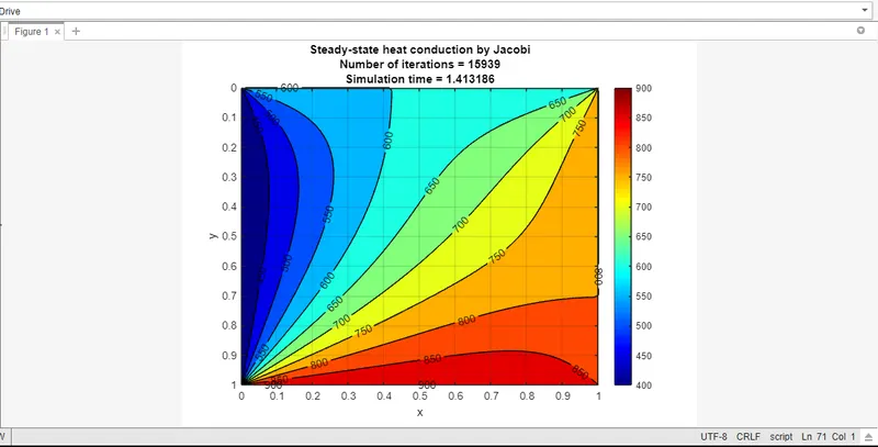
Jacobi Iterative method:

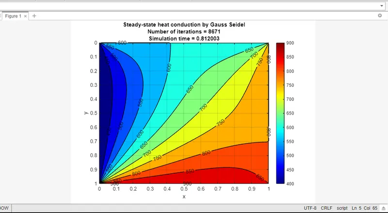
Gauss-Seidel Iterative method:

Successive over relaxation iterative method:

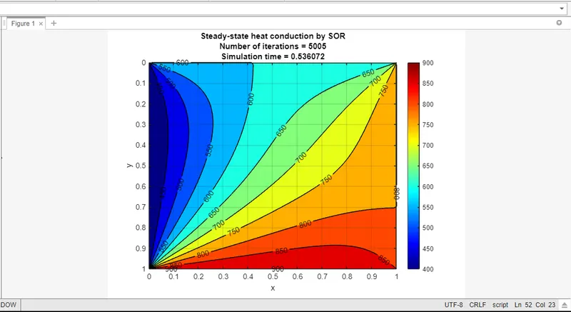
By comparing the convergence rates of all the three methods, SOR converges in a small number of iterations in less simulation time. Here, we conclude the convergence rates by

Jacobi > Gauss-Seidel > SOR.

Unsteady / Transient state 2D heat conduction equation by explicit scheme:

The equations given below for explicit scheme,

`(T_(i,j)^(n+1)-T_(i,j)^n)/(trianglet)-alpha*((T_(i+1,j)-2T_(i,j)+T_(i-1,j))^n/(trianglex^2)+(T_(i,j+1)-2T_(i,j)+T_(i,j-1))^n/(triangley^2))=0`

`T_(i,j)^(n+1)=T_(i,j)^n+(trianglet*alpha)*((T_(i+1,j)-2T_(i,j)+T_(i-1,j))^n/(trianglex^2)+(T_(i,j+1)-2T_(i,j)+T_(i,j-1))^n/(triangley^2))`

`T_(i,j)^(n+1)=T_(i,j)^n+k_1*(T_(i+1,j)-2T_(i,j)+T_(i-1,j))^n+k_2*(T_(i,j+1)-2T_(i,j)+T_(i,j-1))^n`

where `k_1 and k_2` are

`k_1=alpha*(trianglet)/(trianglex^2)`

`k_2=alpha*(trianglet)/(triangley^2)`

MATLAB code for Unsteady state heat conduction by explicit scheme:

clear all
close all
clc

% 2D Unsteady-state heat conduction by explicit method
% Initial conditions
L = 1;
%grid points
nx = 20;
ny = 20;
x = linspace(0, 1, nx);
y = linspace(0, 1, ny);
%grid spacing
dx = x(2) - x(1);
dy = y(2) - y(1);

dt = 1/3000; % Time step
alpha = 1.1; % Thermal diffusivity

% Initial boundary conditions
t = 300 * ones(nx, ny);
t(:, 1) = 400;
t(1, :) = 600;
t(:, ny) = 800;
t(nx, :) = 900;

%temperature at corner points
t(1, 1) = 500;
t(nx, ny) = 850;
t(1, ny) = 700;
t(nx, 1) = 650;

k1 = (alpha * dt) / (dx^2);
k2 = (alpha * dt) / (dy^2);
nt = 800;
CFL = alpha * ((1 / dx^2) + (1 / dy^2)) * dt;

told = t;
tol = 1e-4; % Convergence criteria
error = 9e9;

tic
% Time Loop
for k = 1:nt % Nodal Loop
    for i = 2:nx-1
        for j = 2:ny-1
            term1 = told(i, j);
            term2 = k1 * (told(i+1, j) - 2 * told(i, j) + told(i-1, j));
            term3 = k2 * (told(i, j+1) - 2 * told(i, j) + told(i, j-1));
            t(i, j) = (term1 + term2 + term3);
        end
    end
    told = t;
end
time_end = toc;

% Plotting
contourf(x, y, t, 'ShowText', 'on');
colorbar
colormap(jet);
set(gca, 'ydir', 'reverse')
xlabel('x')
ylabel('y')
text1 = sprintf('Number of time steps = %d', nt);
text2 = sprintf('Simulation time = %f', time_end);
title({'Unsteady-state heat conduction by Explicit Method', text1, text2});
grid on

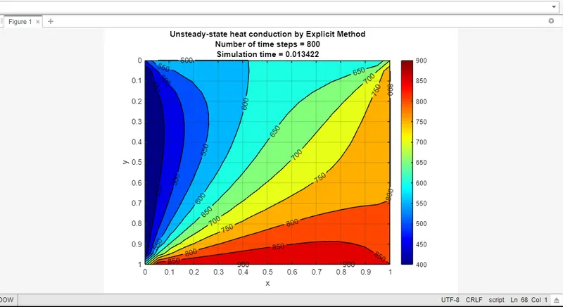
In explicit scheme, the solution converges very fast with less number of iterations.

Unsteady / Transient state 2D heat conduction equation by implicit scheme:

The equations for implicit schemes are given below,

`T_(i,j)^(n+1)=(T_(i,j)^n+k_1*(T_(i+1,j)+T_(i-1,j))^(n+1)+k_2*(T_(i,j+1)+T_(i,j-1))^(n+1))/(1+2k_1+2k_2)`

For Jacobi,

`T_(i,j)^(n+1)=(T_(i,j)^n+k_1*(T_(i+1,j)+T_(i-1,j))^n+k_2*(T_(i,j+1)+T_(i,j-1))^n)/(1+2k_1+2k_2)`

For Gauss-Seidel,

`T_(i,j)^(n+1)=(T_(i,j)^n+k_1*(T_(i+1,j)+T_(i-1,j))^(n+1)+k_2*(T_(i,j+1)+T_(i,j-1))^(n+1))/(1+2k_1+2k_2)`

For SOR,

`T_(i,j)^(n+1)=T_(i,j)^n(1-omega)+omega*((T_(i,j)^n+k_1*(T_(i+1,j)+T_(i-1,j))^(n+1)+k_2*(T_(i,j+1)+T_(i,j-1))^(n+1))/(1+2k_1+2k_2))`

MATLAB code for Unsteady state heat conduction by implicit scheme:

clear all
close all
clc

% 2D Unsteady-state heat conduction
% Initial conditions
L = 1;
%grid points
nx = 20;
ny = 20;
x = linspace(0, 1, nx);
y = linspace(0, 1, ny);
%grid spacing
dx = x(2) - x(1);
dy = y(2) - y(1);

dt = 20; % Time step
alpha = 1.4; % Thermal diffusivity

% Initial boundary conditions
t =300* ones(nx, ny);
t(:, 1) = 400;
t(1, :) = 600;
t(:, ny) = 800;
t(nx, :) = 900;

%temperature at corner points
t(1, 1) = 500;
t(nx, ny) = 850;
t(1, ny) = 700;
t(nx, 1) = 650;

k1 = (alpha * dt) / (dx^2);
k2 = (alpha * dt) / (dy^2);
nt = 1000;
CFL = alpha * ((1 / dx^2) + (1 / dy^2)) * dt;

told = t;
t_prev = told;
tol = 1e-4; % Convergence criteria
error = 9e9;

for iterative_method = 1 % Set the iterative method to Jacobi

if iterative_method ==1
     tic;
     jacobi_iter = 1;
     % Time Loop
       for c = 1:nt
           while (error > tol)
               % Space Loop
             for i = 2:nx-1
                for j = 2:ny-1
                    term1 = (1+(2*k1)+(2*k2))^(-1);
                    term2 = k1*term1;
                    term3 = k2*term1;
                    H = (told(i-1,j) + told(i+1,j));
                    V = (told(i,j-1) + told(i,j+1));
                    t(i,j) = ((t_prev(i,j)*term1) + (H*term2) + (V*term3));
                end
             end
                error = max(max(abs(told - t)));
                told = t;
                jacobi_iter = jacobi_iter + 1;      
           end
           t_prev = t;
       end
         time_end2 = toc;

    % Plotting
    contourf(x, y, t, 'ShowText', 'on');
    colorbar
    colormap(jet);
    set(gca, 'ydir', 'reverse')
    xlabel('x')
    ylabel('y')
    text1 = sprintf('Number of iterations = %d',jacobi_iter);
    text2 = sprintf('Simulation time = %f', time_end2);
    title({'Unsteady-state heat conduction using Jacobi iterative method', text1, text2});
    grid on
end
end

clear all
close all
clc

% 2D Unsteady-state heat conduction using Gauss Seidel
% Initial conditions
L = 1;
%grid points
nx = 20;
ny = 20;
x = linspace(0, 1, nx);
y = linspace(0, 1, ny);
%grid spacing
dx = x(2) - x(1);
dy = y(2) - y(1);

dt = 20; % Time step
alpha = 1.4; % Thermal diffusivity

% Initial boundary conditions
t = ones(nx, ny);
t(:, 1) = 400;
t(1, :) = 600;
t(:, ny) = 800;
t(nx, :) = 900;

%temperature at corner points
t(1, 1) = 500;
t(nx, ny) = 850;
t(1, ny) = 700;
t(nx, 1) = 650;

k1 = (alpha * dt) / (dx^2);
k2 = (alpha * dt) / (dy^2);
nt = 800;
CFL = alpha * ((1 / dx^2) + (1 / dy^2)) * dt;

told = t;
tol = 1e-4; % Convergence criteria
error = 9e9;
t_prev = told;

term_1 = (1 + (2 * k1) + (2 * k2))^-1;
term_2 = k1 * term_1;
term_3 = k2 * term_1;

for iterative_method = 1 % Set the iterative method to Gauss seidel

if iterative_method ==1
     tic;
     GS_iter = 1;
     % Time Loop
       for c = 1:nt
           while (error > tol)
               % Space Loop
             for i = 2:nx-1
                for j = 2:ny-1
                    term1 = (1+(2*k1)+(2*k2))^(-1);
                    term2 = k1*term1;
                    term3 = k2*term1;
                    H = (t(i-1,j) + told(i+1,j));
                    V = (t(i,j-1) + told(i,j+1));
                    t(i,j) = ((t_prev(i,j)*term1) + (H*term2) + (V*term3));
                end
             end
                error = max(max(abs(told - t)));
                told = t;
                GS_iter = GS_iter + 1;      
           end
           t_prev = t;
       end
         time_end2 = toc;

    % Plotting
    contourf(x, y, t, 'ShowText', 'on');
    colorbar
    colormap(jet);
    set(gca, 'ydir', 'reverse')
    xlabel('x')
    ylabel('y')
    text1 = sprintf('Number of iterations = %d',GS_iter)
    text2 = sprintf('Simulation time = %f', time_end2);
    title({'Unsteady-state heat conduction for GS iterative method', text1, text2});
    grid on
end
end

clear all
close all
clc

% 2D Unsteady-state heat conduction USING Succesive over relaxation method
% Initial conditions
L = 1;
%grid points
nx = 20;
ny = 20;
x = linspace(0, 1, nx);
y = linspace(0, 1, ny);
%grid spacing
dx = x(2) - x(1);
dy = y(2) - y(1);

dt = 20; % Time step
alpha = 1.4; % Thermal diffusivity
omega=1.2; %relaxation factor
% Initial boundary conditions
t =300* ones(nx, ny);
t(:, 1) = 400;
t(1, :) = 600;
t(:, ny) = 800;
t(nx, :) = 900;

%temperature at corner points
t(1, 1) = 500;
t(nx, ny) = 850;
t(1, ny) = 700;
t(nx, 1) = 650;

k1 = (alpha * dt) / (dx^2);
k2 = (alpha * dt) / (dy^2);
nt = 1000;
CFL = alpha * ((1 / dx^2) + (1 / dy^2)) * dt;

told = t;
t_prev = told;
tol = 1e-4; % Convergence criteria
error = 9e9;

for iterative_method = 1 % Set the iterative method to SOR

if iterative_method ==1
     tic;
     sor_iter = 1;
     % Time Loop
       for c = 1:nt
           while (error > tol)
               % Space Loop
             for i = 2:nx-1
                for j = 2:ny-1
                    term1 = (1+(2*k1)+(2*k2))^(-1);
                    term2 = k1*term1;
                    term3 = k2*term1;
                    H = (t(i-1,j) + told(i+1,j));
                    V = (t(i,j-1) + told(i,j+1));
                    t(i,j) = (told(i,j)*(1-omega)) + omega*((t_prev(i,j)*term1)+(H*term2) + (V*term3));
                end
             end
                error = max(max(abs(told - t)));
                told = t;
                sor_iter = sor_iter + 1;      
           end
           t_prev = t;
       end
         time_end2 = toc;

    % Plotting
    contourf(x, y, t, 'ShowText', 'on');
    colorbar
    colormap(jet);
    set(gca, 'ydir', 'reverse')
    xlabel('x')
    ylabel('y')
    text1 = sprintf('Number of iterations = %d',sor_iter);
    text2 = sprintf('Simulation time = %f', time_end2);
    title({'Unsteady-state heat conduction using SOR iterative method', text1, text2});
    grid on
end
end

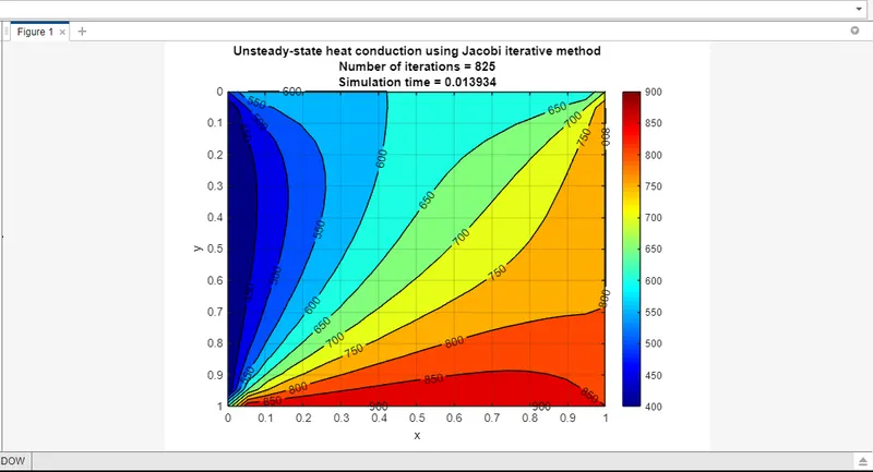
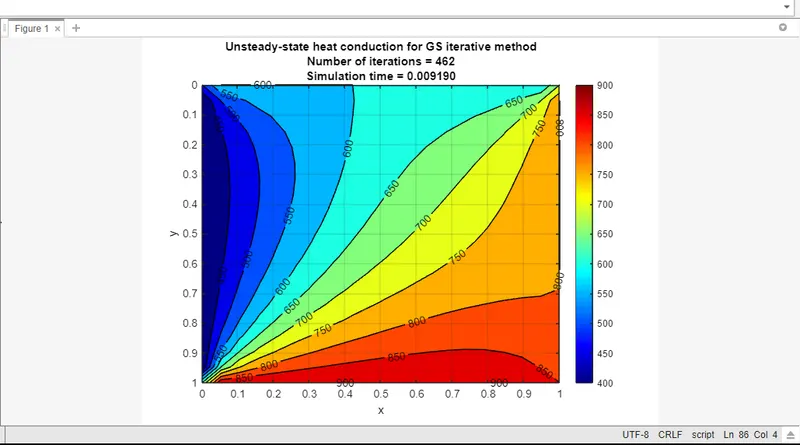
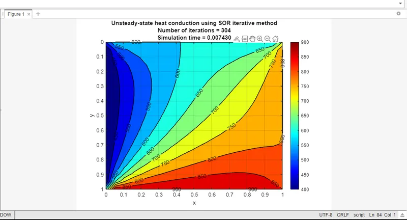
For 2D transient implicit heat conduction equation, SOR gives better convergence rate in less simulation time by comparing other two iterative methods.

Conclusion:

For computational efficiency, explicit scheme is preferred. For accuracy and stability, implicit scheme is preferred. It depends upon the criteria we need.