Week 5 - Genetic Algorithm

Aim : To learn how the genetic alogrithm (ga) code work in matlab

Prior knowledge:

a) What is stalagmite ?

Stalagmites and stalactites are some of the best known cave formations. They are icicle-shaped deposits that form when water dissolves overlying limestone then re-deposits calcium carbonate along the ceilings or floors of underlying caves. Stalactites form along ceilings and hang downward. When stalactites are actively forming, they drip water. Where that water hits the floor, a mound-shaped stalagmite will form.

b) What is a stalagmite function?

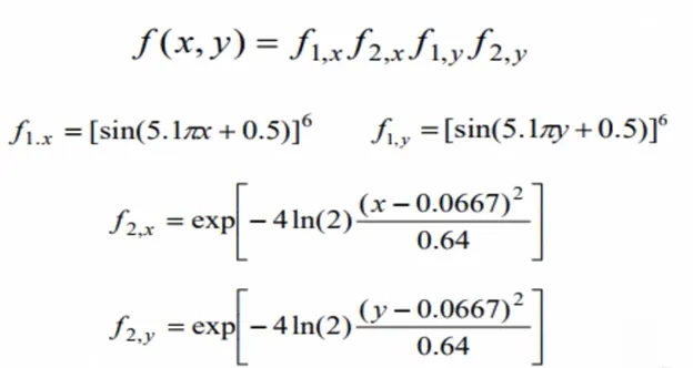
It has two variable that are x and y. if we need to create the program we have to give two inputs to the function so it can solve the function.

c) What is optimization?

In basic term it means the act of making the effective usage of resources. Its an act, process, or methodology of making something (such as a design, system, or decision) as fully perfect, functional, or effective as possible

d) what are the technique used to perform optimization?

there are two type of optimization technique are as follows:

1) deterministic approach: specific rules are used to solve the function and move from one solution to another.

2) stochastic approach: its a probablistic approach, its posses a inherant randomness.

Genetic algorithm is on of them, it a search based optimization method based on the principles of genetics and natural sciences. its can be explained with one phrase 'survival of the fittest'.

its consist of stages the flow chart will explain it in a better way:

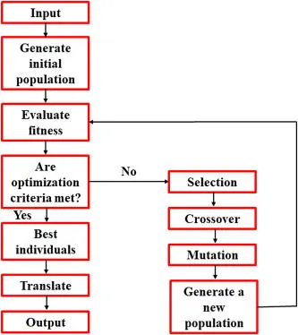
Selection: In this step we select the two input from the sample we have taken for evaluation. selection depends on the fitness value if the elements.

crossover: In this step the selected elements react with each other and new generation is formed which will have the best qualities from both the elements and few other qualities also.

Mutation: In this step we let the newly created element gains new qualities and develop.

your can refer the foloowing articl for more knowledge: Genetic Algorithm explained!! : Skill-Lync

Program codded to solve the given challenge:

clear all
close all
clc

% starting the program from the guven input of value in meters(m)
x=linspace(0,0.6,150); % creating the x array from 0 to 0.6 
y=linspace(0,0.6,150); % creating the y array from 0 to 0.6 
num_cases = 50;        % no of iteration taken to calculate the stalagmite function

% Creating the arrays 
[xx,yy] = meshgrid(x,y); % creating a matrix 

% nested for loop to find the maxima of the given stalagmite
% evaluating the stalagmite function
for i=1:length(xx)
    for j=1:length(yy)
        inp_vec(1)=xx(i,j);
        inp_vec(2)=yy(i,j);
        F(i,j) = stalagmite_func(inp_vec);
    end
end

F=-F;   % so that the graph which we see will provide the maxima 
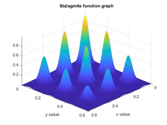
figure(1)
surfc(xx,yy,F) % we will provide the 3d plot 
shading interp % it will provide the smooth graph with no grid line 

title('Stalagmite function graph')
xlabel('x value')
ylabel('y value')
[input, fopt(i)] = ga(@stalagmite_func,2) % call the stalagmite function 


% unbounded ( no limits has been given to x and y value )
tic          % it will start the timer for calculating the time required to execute the 
                    for loop
for i=1:num_cases  % considering only 50 value for calculation
    [input_2, fopt_2(i)] = ga(@stalagmite_func,2); % call the stalagmite function
    x_opt_2(i)= input_2(1); % value of 'x' taken in consideration to calculate the 
                             stalagmite function
    y_opt_2(i)= input_2(2); % value of 'y' taken in consideration to calculate the 
                             stalagmite function
end
fopt_2=-fopt_2;  % ga will provide the minima but we require maxima so minus sign is 
                      used
study_time_1 = toc; % timer will stop and time will be recorded.

%ploting
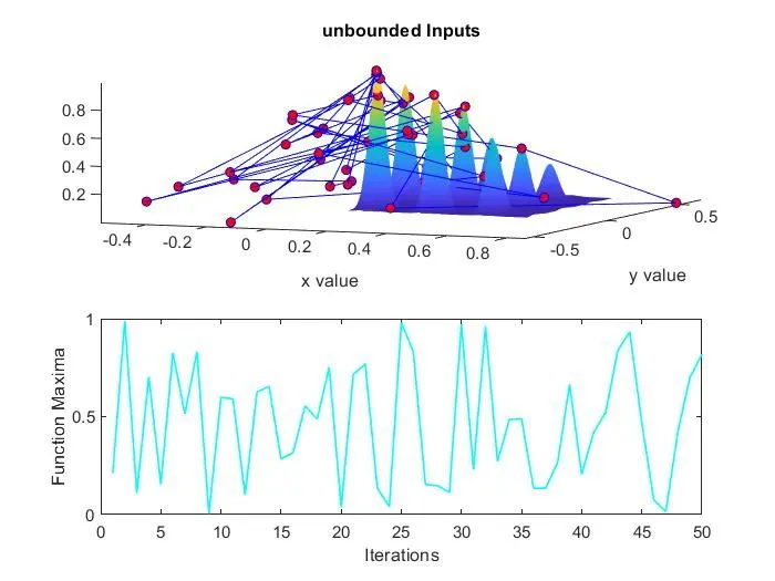
figure(2) 
subplot(2,1,1)
hold on
surfc(xx,yy,F)  
shading interp
xlabel('x value')
ylabel('y value')
plot3(x_opt_2,y_opt_2,fopt_2,'color','b','marker','o','markersize',5,'markerfacecolor','r') % plotting all Local maxima value unbounded
title('unbounded Inputs')
subplot(2,1,2)
plot(fopt_2,'color','c','linewidth',1) 
xlabel('Iterations')
ylabel('Function Maxima')

% bounded input with upper and lower bound
tic
for i=1:num_cases
    [input_3, fopt_3(i)] = ga(@stalagmite_func,2,[],[],[],[],[0;0],[1;1]); 
    x_opt_3(i)= input_3(1);
    y_opt_3(i)= input_3(2);
end
fopt_3=-fopt_3;
study_time_2=toc

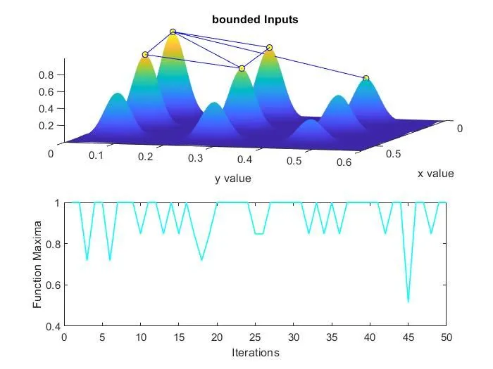
figure(3)
subplot(2,1,1)
hold on
surfc(xx,yy,F)
shading interp
xlabel('x value')
ylabel('y value')
plot3(x_opt_3,y_opt_3,fopt_3,'color','b','marker','o','markersize',5, 'markerfacecolor','y')
title('bounded Inputs')
subplot(2,1,2)
plot(fopt_3,'color','c','linewidth',1)
xlabel('Iterations')
ylabel('Function Maxima')

% bounded input with increasing the population 
options = optimoptions('ga')
options = optimoptions(options,'populationsize',300)
tic
for i=1:num_cases
    [input_4, fopt_4(i)] = ga(@stalagmite_func,2,[],[],[],[],[0;0],[1;1],[],[],options);
    x_opt_4(i)= input_4(1);
    y_opt_4(i)= input_4(2);
end
fopt_4=-fopt_4;
study_time_3=toc

figure(4)
subplot(2,1,1)
hold on
surfc(xx,yy,F)
shading interp
xlabel('x value')
ylabel('y value')
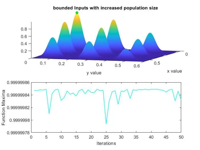
plot3(x_opt_4,y_opt_4,fopt_4,'marker','o','markersize',5,'markerfacecolor','g')
title('bounded Inputs with increased population size ')
subplot(2,1,2)
plot(fopt_4,'color','c','linewidth',1)
xlabel('Iterations')
ylabel('Function Maxima')

Stalagmite Function used to solve the code:

function F = stalagmite_func(inp_vec)
x = inp_vec(1);
y = inp_vec(2);
 f1_x = (sin ( 5.1 * pi * x + 0.5))^6;
 f1_y = (sin ( 5.1 * pi * y + 0.5))^6;
 f2_x = exp (( -4 * log(2) * (x - 0.0667)^2 )/ (0.64));
 f2_y = exp (( -4 * log(2) * (y - 0.0667)^2 )/ (0.64));
 F = -(f1_x*f1_y*f2_x*f2_y);
end

Syntax used in the program:

1) x = ga(fun,nvars) finds a local unconstrained minimum, x, to the objective function, fun. nvars is the dimension (number of design variables) of fun.

[input, fopt(i)] = ga(@stalagmite_func,2) @ is a anaynmous function operator, 'stalagmite_func' if a function file in which stalagmite function is stored and '2' is the no of variable used in the function file.

2) x = ga(fun,nvars,A,b,Aeq,beq,lb,ub) defines a set of lower and upper bounds on the design variables, x, so that a solution is found in the range lb (lower bound=0) ≤ x ≤ ub (upper bound=1) . (Set Aeq=[] and beq=[] if no linear equalities exist.)

[input_3, fopt_3(i)] = ga(@stalagmite_func,2,[],[],[],[],[0;0],[1;1]);

Return an empty entry [] for a nonexistent constraint

{0,0] lower bound of x and y, [1,1] upper bound of x and y.

3)x = ga(fun,nvars,A,b,Aeq,beq,lb,ub,nonlcon,options) minimizes with the default optimization parameters replaced by values in options. (Set nonlcon=[] if no nonlinear constraints exist.) Create options using optimoptions.

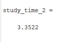
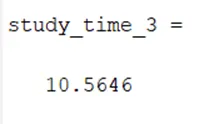
Output after evaluation in command window:

.

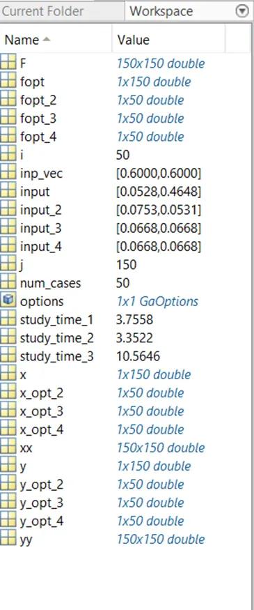
Value Shown in workspace:

Plots:

Conclusion:

In unbounded solution: The local maxima out of the range also has been shown in the first plot and there are many maxima seen in the second plot.

In bounded solution: There are less local Maxima out of the range but this time they are bounded between 0 and 1 for both x and y axis.

In fig(4), the population has been increased so when we run the function we get only one maxima.