Week 4.1 - Solving second order ODEs

Link of the animation:https://drive.google.com/file/d/1_v3N59j0HsyagYNyZykPWlBZQ2mnlWIC/view?usp=share_link

program required to create that animation:

clear all
close all
clc

%input 
l = 1                        % length of the rod in m
m = 1                         % weight of the ball in kg
g = 9.81                     % gravitional acceleration in m/sec^2
b = 0.05                     % damping coefficient

%initial condition
theta_0 = [0;3]; % value of displacment and angular velocity at the initial condition 

%time points
t_span = linspace(0,20,500); % a array of time between 0 to 20 sec is been created 

%solve ode
[t x] = ode45(@(t,theta) ode_func(t_span,theta,b,g,l,m), t_span,theta_0);

%plotting
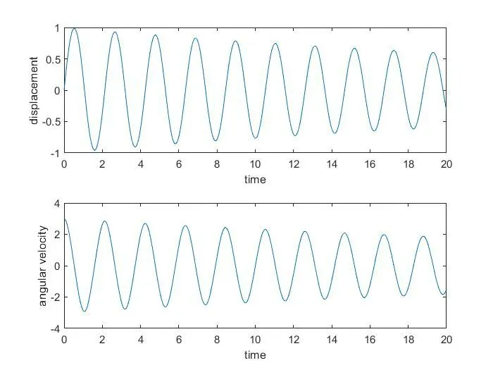
subplot(2,1,1)  % divide the figure in to 2 rows and 1 coloum and place the axis in the first row
plot(t,x(:,1))  % ploting the time on x axis and displacement on y axis. (:,1) selecting all value of rows and 1st column
hold on
ylabel('displacement')
xlabel('time')
subplot(2,1,2)  % divide the figure in to 2 rows and 1 coloum and place the axis in the second row
plot(t,x(:,2))  % ploting the time on x axis and displacement on y axis. (:,1) selecting all value of rows and 2nd column
ylabel('angular velocity')
xlabel('time')

%ANIMATION
x0 = 0
y0 = 0
ct = 1;
for i = 1:length(t)
    x1 = l*sin(x(i,1));          % it will select all the value of displacement for 
                                   calculating the value of x1
    y1 = -l*cos(x(i,l));         % it will select all the value of displacement for 
                                   calculating the value of y1
    figure(2)
    plot([-1 1],[0 0],'linewidth',6,'color','g');   % it will create the support rod
    axis([-2 2 -2 2]);
    line([x0 x1],[y0 y1],'linewidth',2,'color','b'); % it will create the connecting rod
    hold on;
    plot(x0,y0,'o','markersize',3,'markerfacecolor','y');  % its used to show the fixed 
                                                              pointer
    plot(x1,y1,'o','markersize',20,'markerfacecolor','r'); % its used to create the ball
    title('Damping of simple Pendulum');
    legend('support rod','length of pendulum','fixed point','Body of pendulum');
    grid on;
    hold off;
    M(ct) = getframe(gcf);
    ct = ct+1;
end
movie(M)                        % with the help of this command we can create animation
videofile = VideoWriter('second order ode.avi','Uncompressed AVI') % naming the file and 
                                                          specifying the format of vedio
open(videofile)
writeVideo(videofile,M)          % it will create the vedio file from all the frame we 
                                       collected by excuting the line35
close(videofile)

Explanation:-

1) input are specified which is required to solve the differential equation.

2) [t x] = ode45(@(t,theta) ode_func(t_span,theta,b,g,l,m), t_span,theta_0);

"[t x]":- this will be the output we will receive after solving the differancial equation.'t' time and 'x' will have two colums 1st column will be displacement and 2nd column will be angular velocity.

"ode45":- we have to yse theis code for solving the ordinary diffential equation

"@(t,theta)":- @ is a ananyomous function , 't' and 'theta' will the input of that function

"ode_func(t_span,theta,b,g,l,m),":- 'ode_func' function caller, '(t_span,theta,b,g,l,m)' input to solve the function specified in the question

"t_span,theta_0":- this will be arrays from which value will be taken to solve the equation

Functional Program required to solve the ode:

function [dtheta_dt] = ode_func(t,theta,b,g,l,m) 

theta1 =  theta(1)
theta2 =  theta(2)
dtheta1_dt = theta(2);             % derevative of theta1 will be equal to theta2
dtheta2_dt = -(b/m)*theta2 - (g/l)*sin(theta1); 
dtheta_dt = [dtheta1_dt; dtheta2_dt]; 
end

Plot after complete excution of the program:-