Week 5 - Genetic Algorithm
PROBLEM DEFINITION;
Try to understand the concept of genetic algorithm by referring to varius sources before you attend this challenge. Look out for information regarding stalagmite function and ways to optimise it.
- Write a code in MATLAB to optimise the stalagmite function and find the global maxima of the function.
- Clearly expalin the concept of genetic algorithm in your own words and also explain the syntax for ga in MATLAB in your report.
- Make sure that your code gives the same output, even if it is made to run several times.
- Plot graphs for all 3 studies and for F maximum vs no. of iterations. Title and axes labels are a must, legends could be shown if necessary.
The presentation of your code will be taken into consideration while grading. Labeling sections of your code is appreciated.
Content expected in the report:
- Step-wise explanation of your code.
- Mention the errors while programming.
- Steps taken to overcome those errors.
- Screenshots showing errors thrown in command window.
WHAT IS OPTIMIZATION?
Optimization is the process of selection from the set of values for the imposed targets and constraints.
Processes handling many parameters where it intrgrated with each other and affects one another in all aspects.
It has been very difficult to manage and select the appropriate range of values for the defined targets and constraints.
To make this process ease optimization techniques helps us to find a way to get the base out of it.
GENETIC ALGORITHM;
> Genetic algorithm is an optimization process which is used to solve the non-linear or non-diffrentiable optimization problem.
> Uses concept from evolutioary biology to switch from global minima to optimization problem.
> Start with an initial generation of candidiate solution that are tested against the objective function.
> subsquent genertion evolve from the first through selection , crossover and mutation.
> SELECTION; it defined as the selection of the person for the next generation using fitness fnction which will be based on the fitness value.
> CROSS OVER; Cross over enables the algorithm to extract the best character from the diffrent individuals and recombine them in to potentially superior children.
> mutation; Mutation adds to the diversity of the population and thereby increases the likelihood that the algorithm will generate individuals with better fitness values.
SYNTAX of GA.
Find minimum of function using genetic algorithm.
x = ga(fun,nvars)
x = ga(fun,nvars,A,b)
x = ga(fun,nvars,A,b,Aeq,beq)
x = ga(fun,nvars,A,b,Aeq,beq,lb,ub)
x = ga(fun,nvars,A,b,Aeq,beq,lb,ub,nonlcon)
x = ga(fun,nvars,A,b,Aeq,beq,lb,ub,nonlcon,options)
fun > objective function
nvars > number of variables specified as positive integer.
A,b > linear inequality constraints.(A > real matrix, b > real vector)
Aeq,Beq > Linear equality constraints.(A > real matrix, b > real vector)
lb,ub > lower bounds and upper bounds.
nonlcon > Nonlinear contraints.
options > optimization options.
OPTIMOPTIONS SYNTAX;
optimoptions
Create optimization optionscollapse all in page
Syntax
options = optimoptions(SolverName)
options = optimoptions(SolverName,Name,Value)
options = optimoptions(oldoptions,Name,Value)
options = optimoptions(SolverName,oldoptions)
options = optimoptions(prob)
options = optimoptions(prob,Name,Value)
SCRIPTING THE OBJECTIVE FUNCTION;
> This describes the stalagmite function.
> This function creates the contour of peaks for the defined input variables with suitable range.
> It is one of the test function which is used to validte the performance characteristic of the optimization algorithms.
> There are mainly three studies those we have to perform in this problem.
1) UNBOUNDED CASE;
> Here in the ga the lower and upper bounds are not defined.
> Having a high probability of getting the inaccurate results.
2) Bounded study;
Here in the ga syntax the lower nd upper bounds are defined.
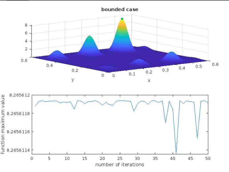
With defined bounds of x from 0 to 0.6 and bounds of y from 0 to 0.6 results in better optimization.
3) Bounded ga study with population size.
> POpualtion size denotes the number of data points initialized in the space for simulation.
> The default popualation size for ga solver is 50.
> Population size can be uses as a feature using "options" in the ga syntax.
> Increase the popualtion size until the single optimum point is achieved.
> INcreasing population size will increase the simulation time.
PROGRAM CODE FOR GENETIC ALGORITHM FOR GETTING THE SINGLE OPTIMUM POINT WHICH WILL GIVE THE MAXIMUM VALUE FOR THE FUNCTION.
clear all
close all
clc

x = linspace(0,0.6,150);

y = linspace(0,0.6,150);

[xx,yy] = meshgrid(x,y);

for i = 1:length(xx)
    for j = 1:length(yy)

        z(1) = xx(i,j);
        z(2) = yy(i,j);


        f(i,j) = stalagmite(z);

    end

end

figure(1)
surfc(xx,yy,-f)
shading interp

% study 1 unbounded case.

num_cases = 50;

tic

for i = 1:num_cases

    [z, fopt(i)] = ga(@stalagmite, 2);

    x_opt(i) = z(1);
    y_opt(i) = z(2);


end

study_one_time = toc;

% plotting the graph

figure(2)
subplot(2,1,1);
surfc(xx,yy,-f);
hold on

shading interp

 plot3(x_opt,y_opt,-fopt,'marker','o','markersize',5,'MarkerFaceColor','g')

title('unbounded case')
xlabel('x');
ylabel('y');

grid on;
subplot(2,1,2);
plot(-fopt);
xlabel('number of iterations');
ylabel('function maximum value');


%
% % study 2 bounded case with lower and upper bounds.

num_cases = 50;

tic

for i = 1:num_cases

    [z,fopt(i)] = ga(@stalagmite, 2,[],[],[],[],[0,0],[0.6,0.6]);

    x_opt(i) = z(1);
    y_opt(i) = z(2);


end

study_one_time = toc;

% plotting the graph

figure(3)
subplot(2,1,1);
surfc(xx,yy,-f);
hold on

shading interp


plot3(x_opt,y_opt,-fopt,'marker','o','markersize',5,'MarkerFaceColor','g');

title('bounded case');
xlabel('x');
ylabel('y');

grid on;
subplot(2,1,2);
plot(-fopt);
xlabel('number of iterations');
ylabel('function maximum value');
%
%
% % study 3 bounded case with lower and upper bounds. with population size.

% modifying the population size

options = optimoptions('ga','PopulationSize',500);

num_cases = 50;

tic

for i = 1:num_cases

    [z,fopt(i)] = ga(@stalagmite, 2,[],[],[],[],[0,0],[0.6,0.6],[],[],options);

    x_opt(i) = z(1);
    y_opt(i) = z(2);


end

study_one_time = toc;
%
% % plotting the graph for incraesed population size i,e,500

figure(4)
subplot(2,1,1);
surfc(xx,yy,-f);
hold on

shading interp


plot3(x_opt,y_opt,-fopt,'marker','o','markersize',5,'MarkerFaceColor','g');

title('bounded case');
xlabel('x');
ylabel('y');

grid on;
subplot(2,1,2);
plot(-fopt);
xlabel('number of iterations');
ylabel('function maximum value');
PLOTS;
FIGURE 1 ;
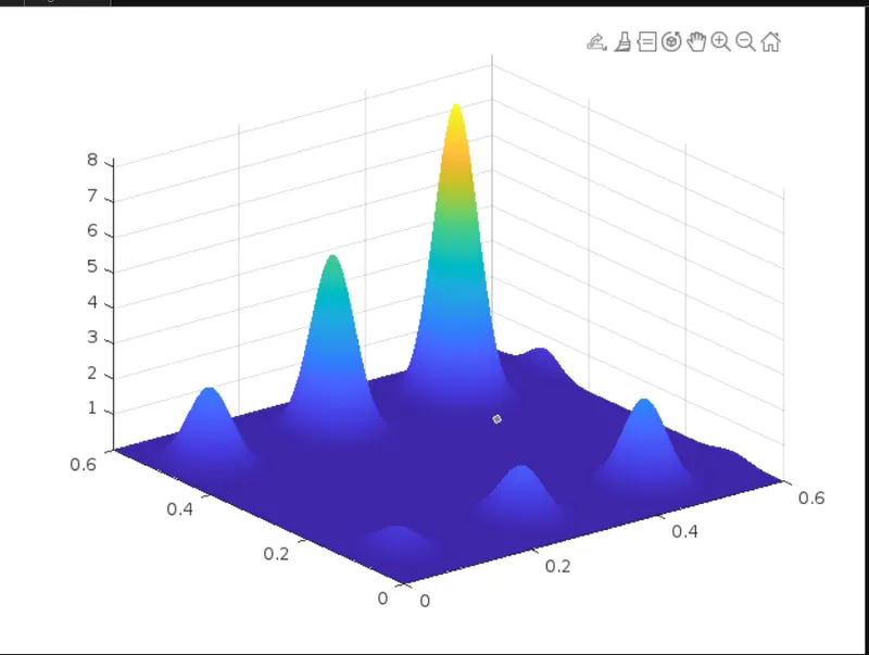
FIGURE(2)
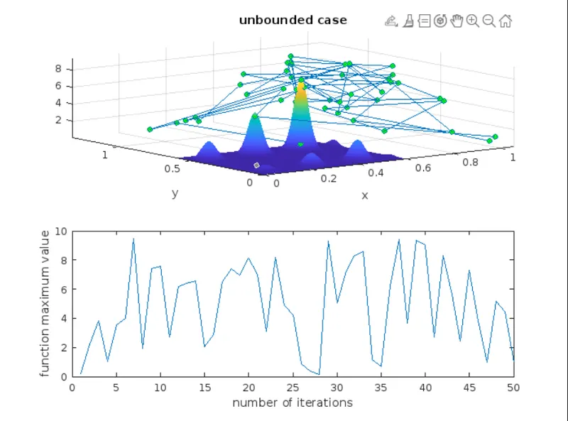
FIGURE(3)
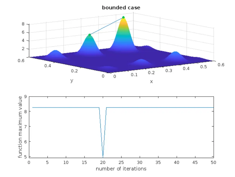
FIGURE(4)