Week 5 - Curve fitting
Meaning of "popt" and "pcov":
“popt” here stands for the optimized parameters of the model function that best fit the given data. “pcov” is the other output from the “curve_fit” function, the covariance matrix. It’s a square matrix where the diagonal elements represent the variance of the parameters and the off-diagonal elements represent the covariance between pairs of parameters. A positive covariance indicates that the parameters tend to vary together (i.e., if one increases, the other tends to increase as well). A negative covariance indicates an inverse relationship (one parameter increases while the other decreases).
What "np.array(temperature)" does:
“np.temperature” is an ‘ndarray’ that stores the values of the temperature read from the file for curve fitting and plotting. In the reference video, the ‘ndarray’ allows us to pass the entire set of values for temperatures read from the file into the defined function “func” to get the corresponding values of the “`C_p`” according to the fitted function. The values of “`C_p`” are also stored in an ‘ndarray’. This makes future calculations and plotting very convenient.
Meaning of "*" in "*popt":
When calling a function, the single asterisk “*” is used to unpack an iterable (e.g., a list or tuple) into separate arguments. So here, ‘*popt’ unpacks the optimised parametrs as input variables into the function “func”.
What need to be done to improve the results from curve fitting:
A higher order numerical model function yields the more accurately fitted curve. As seen from the resulting plots, the curve from the ‘biquadratic’ model fits the best. However, a higher order model may not always generate the best fit as the risk of “overfitting” (occurs when a model fits the training data too closely, capturing not only the underlying pattern but also the noise or random fluctuations in the data) increases. A way to counter this risk is to work with large sample sizes. This reduces the risk of overfitting.
The code: (with comments explaining each step)
import numpy as np
import matplotlib.pyplot as plt
from scipy.optimize import curve_fit
#Defining the linear model:
def linear_model(t,a,b):
return (a*t+b)
#Defining the cubic model:
def cubic_model(t,l,m,n,o):
return(l*pow(t,3)+m*pow(t,2)+n*t+o)
def biquadratic_model(t,d,e,f,g,h):
return(d*pow(t,4)+e*pow(t,3)+f*pow(t,2)+g*t+h)
#Dedfining a functiion to calculate the residual:
def residual(cp_dat,modelledVal):
return abs(cp_dat-modelledVal)
#Function to read the data from the file:
def read_file():
#Initialising empty arrays for temperatures/Cp
temp=[]
cp=[]
for el in open("data","r"):
values=el.split(",")
temp.append(float(values[0]))
cp.append(float(values[1]))
return [temp,cp]
#Reading the data from the supplied file:
temp,cp=read_file()
params_linear,covar_linear=curve_fit(linear_model,temp,cp)
#'params_linear' are the optimised parameters obtained from the curve fitting using the linear function
#'covar_linear' is the resulting covariance matrix
fit_linear=linear_model(np.array(temp),*params_linear) #fit_linear will be an 'ndarray'
params_cubic,covar_cubic=curve_fit(cubic_model,temp,cp)
#'params_cubic' are the optimised parameters obtained from the curve fitting using the cubic function
#'covar_cubic' is the resulting covariance matrix
fit_cubic=cubic_model(np.array(temp),*params_cubic) #fit_cubic will be an 'ndarray'
params_biquadratic,covar_biquadratic=curve_fit(biquadratic_model,temp,cp)
#'params_cubic' are the optimised parameters obtained from the curve fitting using the cubic function
#'covar_cubic' is the resulting covariance matrix
fit_biquadratic=biquadratic_model(np.array(temp),*params_biquadratic) #fit_quadratic will be an 'ndarray'
#calculating residuals:(an empirical way to measure how good the fitting is)
residual_linear=residual(np.array(cp),np.array(fit_linear))
residual_cubic=residual(np.array(cp),np.array(fit_cubic))
residual_biquadratic=residual(np.array(cp),np.array(fit_biquadratic))
#Plotting the actual data with the fitted curves;
plt.figure()
plt.plot(temp,cp,color='blue')
plt.plot(temp,fit_linear,color='red')
plt.title("Fitted Curves (using Linear Model) vs Actual Data")
plt.xlabel("Temperatures")
plt.ylabel("C_p")
plt.legend(['Actual Data','Linear Model'])
plt.show()
plt.figure()
plt.plot(temp,cp,color='blue')
plt.plot(temp,fit_cubic,color='green')
plt.title("Fitted Curves (using Cubic Model) vs Actual Data")
plt.xlabel("Temperatures")
plt.ylabel("C_p")
plt.legend(['Actual Data','Cubic Model'])
plt.show()
plt.figure()
plt.plot(temp,cp,color='blue')
plt.plot(temp,fit_biquadratic,color='yellow')
plt.title("Fitted Curves (using Biuadratic Model) vs Actual Data")
plt.xlabel("Temperatures")
plt.ylabel("C_p")
plt.legend(['Actual Data','Biquadratic Model'])
plt.show()
plt.figure()
plt.plot(temp,residual_linear,color='red')
plt.plot(temp,residual_cubic,color='green')
plt.plot(temp,residual_biquadratic,color='yellow')
plt.title("Residuals")
plt.xlabel("Temperatures")
plt.ylabel("Residuals")
plt.legend(['Linear Model','Cubic Model','Biquadratic Model'])
plt.show()
Results and their analysis:
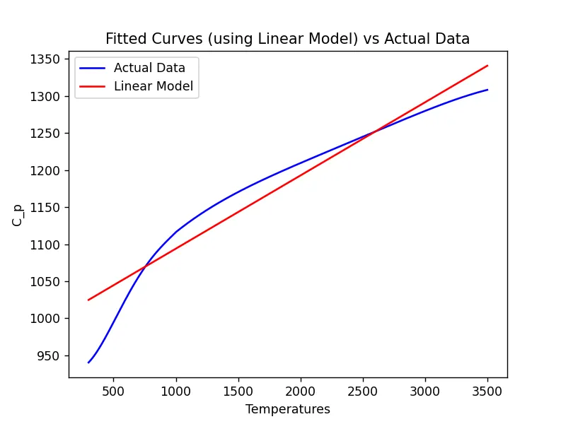
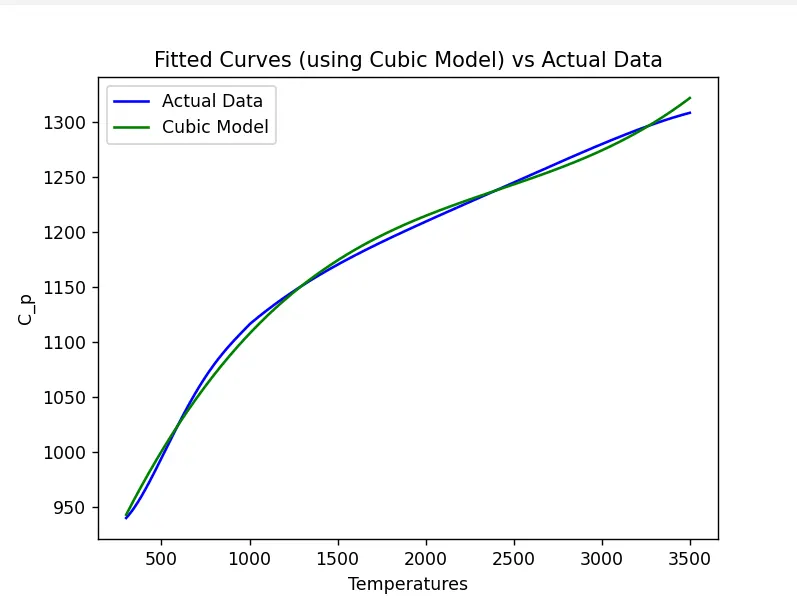
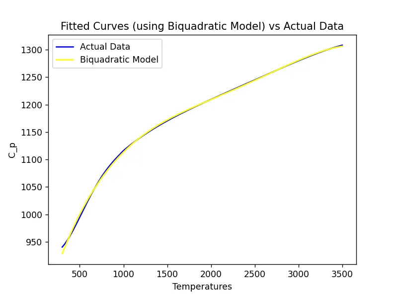
From a basic inspection, it was evident that the biquadratic model produced the best results. The curve from the cubic model did not fit as well. The linear model produced the worst results.
Emperically evaluating the fit:
A good empirical measure to see how well the curve has been fit is by “Residual Analysis”. The residual is the absolute value of the difference of the actual data with the values obtained from the fitted curve. The code also plots the residuals for each of the model functions.
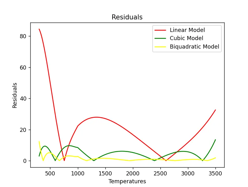
Residual analysis also supports that the biquadratic model produced the best results.The residuals from the cubic and the biquadratic model are not very high. The residuals from the cubic model however oscillates more in comparison to those from the biquadratic model, thus emperically indicating it's better fit. The residuals from the linear model are very high in magnitude and also fluctuale a lot. This indicates the bad fit from the linear model.