Week 5 - Curve fitting

AIM: Curve Fitting

Objective: The objective of this project is to study about curve fit and its use in programing. And explain all the codes and write down the answer of each questions.

These questions are to be explained in this project

• What does popt and pcov mean?

• What does np.array(temperature) do?

• What does the * in *popt mean?

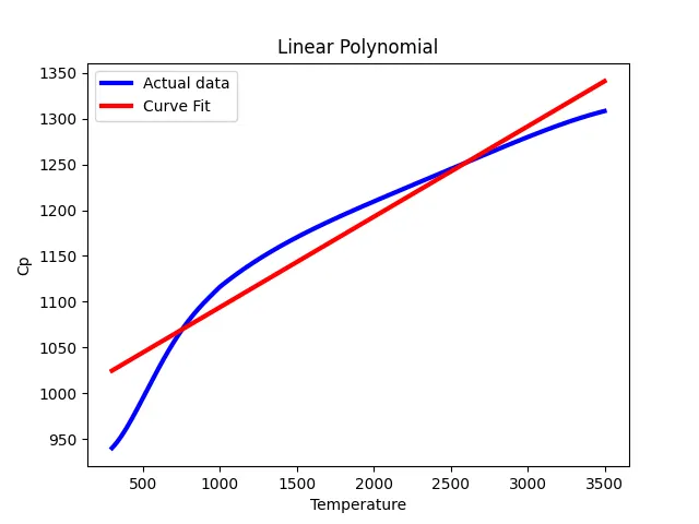
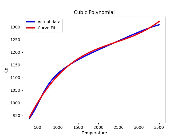
• Write code to fit a linear and cubic polynomial for the Cp data. Explain if your results are good or bad.

• What needs to be done in order to make the curve fit perfect?

• Show empirically as to how well your curve has been fit.

Curve Fitting

"Curve fitting is the process of finding a mathematical function in an analytic form that best fits this set of data."

Generally, curve fitting falls into two main categories based on how we handle the observed data:

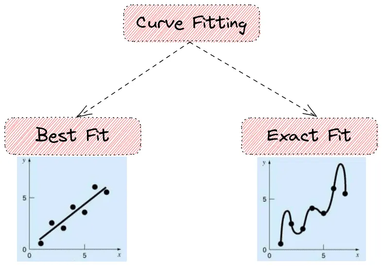
Best Fit:

Here, we assume that the measured data points are noisy. So, we don’t want to fit a curve that intercepts every data point. Our goal is to learn a function that minimizes some predefined error on the given data points.

The simplest best fit method is Linear regression, where the curve is a straight line. More formally, we have the parametric function`y = ax +b` were `a` is the slope and `b` is the intercept and a set of samples `(x1,y1),(x2,y2),(x3,y3)......(Xn,Yn)`. Our goal is to learn the values of `a` and `b` to minimize an error criterion on the given samples.

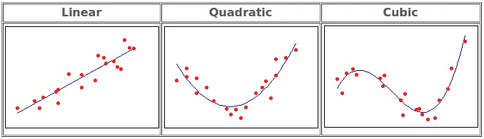
More generally, polynomial regression refers to the case that we want to fit a polynomial of a specific order `d` (degree) to our data:

• linear when `d = 1 : y = ax+b`
• quadratic when `d = 2: y = ax^2 + bx +c`
• cubic when `d = 3: y = ax^3 + bx^2+cx+d`

Where, `d =`degree of polynomial

In the functions above, we can observe that each time the parameters we want to learn are equal to `d+1`. Below, we can see some examples of curve fitting using different functions:

Exact Fit:

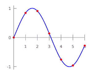
In this case, we assume that the given samples are not noisy, and we want to learn a curve that passes through each point. It is useful in cases we want to derive finite-difference approximations or to find minimums, maximums, and zero crossings of a function.

In the figure below, we can see an example of an exact fit using polynomial interpolation.

Given Data:

Here is the given data of steam table where Heat Capacity (cp) is dependent upon changes in Temperature (T). The dependent variable is Heat Capacity (cp) and independent variable is Temperature (T).

Python code to fit a linear and cubic polynomial for the Cp data

Procedure and Explaination:

Step-1: Before writing the program first we have to import command to import libraries which will be used in mathematical operation and plotting.

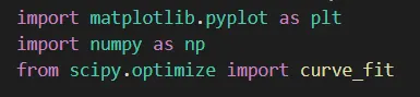
Function of the libraries is:

• matplotlib library for plotting graphs
• numpy library to use np as command which returns evenly spaced samples
• Curve_fit is imported from scipy.optimize library to give curve accoding to Cp data.

Step-2: Define function to fit a linear and polynomial for the Cp data

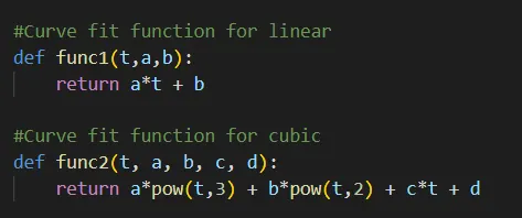
Here we create function for each polynomial equation where the first function is linear polynomial `f(t) = y = at +b`and second function is cubic polynomial `f(t) = y = ax^3 +bt^2+ct+d`.

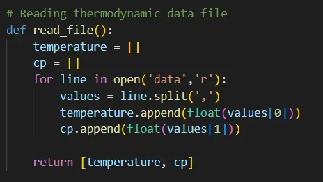
Step-3: Reading thermodynamic data file

After setting function we will call the cp and temperature data from data file by defining function and applying for we are going to store each data line by line in their respective array. To store their value separately split line by "," in two part assign first value "value 0" as temperature and next value "value 1" as cp.

Use return to read all the line step by step and store values in empty array accordingly.

Step-4: Program for curve fitting

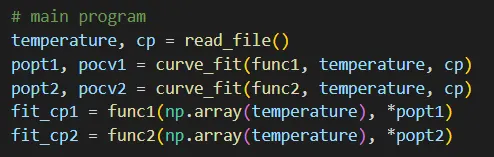
From here, we can start our main coding by curve fitting

• We are going to call the read_file() function to call cp and temperatures values which is out actual value using this value we are going to find out our curve fit.
• Here we are using scipy library for optimization for best curve fit.
• func - the callable function that we created using different type of polynomial equation. xdata- the The independent variable where the data is measured. Should usually be an M-length sequence or an (k,M)-shaped array for functions with k predictors, but can actually be any object. ydata - The dependent data, a length M array - nominally f(xdata,…)
• popt (1-D array) - Optimal values for the parameters so that the sum of the squared residuals of f(xdata, *popt)-ydata in minimize. pcov(2-D array) - The estimated covariance of popt. The diagonals provide the variance of the parameter estimate.
• Predicted array (for curve fit) by using function is calculated by using xdata and optimum value for the co-efficient of the equation. In this case, '*' in '*popt' is used to pass all the required positional arguments to determine function means pass all the coefficients value from function.
• Here we write code for linear polynomial as well as cubic polynomial.

Step-5: Creating Plot

After defining all the terms we need the output so to do that we are using the plot command and plot the graph. Plotting temperature vs specific heat(cp) and temperature vs fit_cp for each polynomial equation.

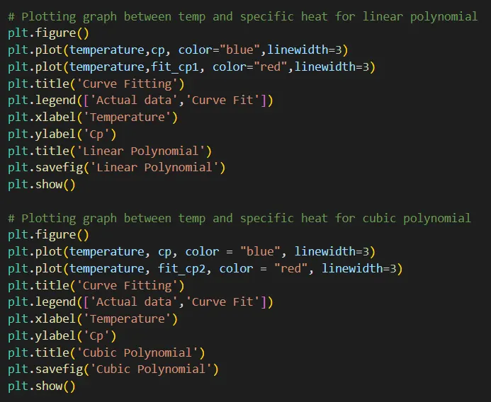
After properly arranging the program we get out the desired program.

Python Program for Curve Fit

CODE:

"""

Curve Fitting using Polynomial equations

"""

import matplotlib.pyplot as plt

import numpy as np

from scipy.optimize import curve_fit

#Curve fit function for linear

def func1(t,a,b):

return a*t + b

#Curve fit function for cubic

def func2(t, a, b, c, d):

return a*pow(t,3) + b*pow(t,2) + c*t + d

# Reading thermodynamic data file

def read_file():

temperature = []

cp = []

for line in open('data','r'):

values = line.split(',')

temperature.append(float(values[0]))

cp.append(float(values[1]))

return [temperature, cp]

# main program

temperature, cp = read_file()

popt1, pocv1 = curve_fit(func1, temperature, cp)

popt2, pocv2 = curve_fit(func2, temperature, cp)

fit_cp1 = func1(np.array(temperature), *popt1)

fit_cp2 = func2(np.array(temperature), *popt2)

# Plotting graph between temp and specific heat for linear polynomial

plt.figure()

plt.plot(temperature,cp,,linewidth=3)

plt.plot(temperature,fit_cp1,,linewidth=3)

plt.title('Curve Fitting')

plt.legend(['Actual data','Curve Fit'])

plt.xlabel('Temperature')

plt.ylabel('Cp')

plt.title('Linear Polynomial')

plt.savefig('Linear Polynomial')

plt.show()

# Plotting graph between temp and specific heat for cubic polynomial

plt.figure()

plt.plot(temperature, cp, color = "blue", linewidth=3)

plt.plot(temperature, fit_cp2, color = "red", linewidth=3)

plt.title('Curve Fitting')

plt.legend(['Actual data','Curve Fit'])

plt.xlabel('Temperature')

plt.ylabel('Cp')

plt.title('Cubic Polynomial')

plt.savefig('Cubic Polynomial')

plt.show()

Output Result:

Curve fitting using Linear Polynomial Curve Fitting using Cubic Polynomial

Here we see in the above figure Cubic polynomial is best fit curve in respective of linear polynomial.

Now we move to the Question answer session

(1) What does popt and pcov mean?

popt (1-D array) - Optimal values for the parameters so that the sum of the squared residuals of f(xdata, *popt)-ydata in minimize.

Its decide the value of co-efficient for a polynomial taken for the approximation of the real data so that the ‘list square method’ of error regression estimation is satisfied.

Pcov(2-D array) - The estimated covariance of popt. The diagonals provide the variance of the parameter estimate.

In other words, pcov decides the covariance for the given optimum values for the curve, which in our case is coefficients of an approximation polynomial.

(2) What does np.array(temperature) do?

np.array(temperature) is the function in numpy library to feed the temperature array or data from the data file with their coefficient values to predict cp (Specific heat value) by passing those value through polynomial function or equation.

(3) What does the * in *popt mean?

Predicted array (for curve fitting) by using function is calculated by using xdata and optimum value for the co-efficient of the equation. In this case, '*' in '*popt' is used to pass all the required positional arguments to determine function means pass all the coefficients value from function.

*popt feeds the value of the optimum coefficient obtained by the least squre method of error regression. Curve_fit function generates optimum parameter value for a given data set then stores it inside output called popt. Which is then use as a function handle for calculating predicted cp value.

(4) Write code to fit a linear and cubic polynomial for the Cp data. Explain if your results are good or bad.

Python code for this polynomial equation is shown above

Result:

Curve fitting using Linear Polynomial Curve Fitting using Cubic Polynomial

Here from above plot generated by python program we can see that in Linear curve fit - curve fit data is different from actual data so it is not best fit according to the actual data. But in Cubic curve fit - curve fit data almost going to parallel with actual data. So as per result we can say that the curve fit getting better as we are increasing the degree of polynomial in the equation and in order to reduce more errors in curve fit we can also use higher degree of polynomial equation which are giving better results.

(5) What needs to be done in order to make the curve fit perfect?

As we observe and study from above graph we can minimize the error and curve fit variation by increasing the order of equation to n+1 degree polynomial.

(6) Show empirically as to how well your curve has been fit

From the above plot we can see that when we increase the degree of polynomial curve getting better and also reduce the error.

CONCLUSION

• Observation based on output plots and figure, we get to know that, errors in the curve fit can be minimize by implementing higher degree polynomial.
• Finally, understood the implementation of scipy.optimize.curve_fit from scipy library