Project 2

PROJECT ON FORWARD ENERGY-BASED FUEL CONSUMPTION MODEL OF A P1 HYBRID VEHICLE

OBJECTIVE:

To develop a forward energy based fuel consumption model of a P1 hybrid vehicle usinig MATLAB/Simulink. Estimating the fuel consumption of P1 Hybrid Drive for different drive cycle and also to compare with Hybrid Drive vehicle and Conventional vehicle.

INTRODUCTION:

With global declination the fossial fuel and tight emission norms by the government of respective country has made an emergency to increase the fuel economy of the vehicles. In the view of above mentioned problem a technology called Hybrid Electric Vehicle (HEV) has immersed and is capable of addressing the above mentioned problem.The key in the technology is the use of another propulsion system which consist of battery and electric motor. Battery is used as energy storage device while motor is used as an electric torque actuator. Thus, this extra drivetrain allows the greater flexibility for engine operation as well as fulfilllment of the power request delivered by the wheel. Surprisingly in early days, ICE engineering was less advanced than electric motor engineeering.

When compared to conventional power train, Hybrid electric vehicle powertrain gives numerous advantages. The use of electric motor able the downsizing of the internal combustion engine with fulfilment of power request by the wheel. With electric motor hybrid power train enables us to captures the waste kinetic energy while braking to electric energy via. the features named as regenerative braking. Due to this sorts of features an optimal control strategies has to be developed for overall smooth performance of the vehicle.

There are many different control strategiess used in hybrid vehicle

And the inputs provide for the hybrid electric vehicle control unit is

• Battery SOC
• Vehicle Speed and Power demand
• Vehicle acceleration
• Present road load
• Braking etc.

Based on the above mentioned input the controller decides on which mode the vehicle needs to be in. The different modes in a HEV are as follow :

• Engine alone mode
• Electric motor alone
• Assist mode( Both motor and engine operate)
• Trickle charging mode (Some Power of the engine is used to charge battery)
• Regenerative braking

In this project P1 hybrid vehicle is model by considering forward energy based model. The control strategies used for this model is rule-based control strategy. In P1 hybrid vehicle, battery and motor is integrated with the engine flywheel which enables the system for idle start stop and regenerative braking. In rule-based control strategy the control rule are frequently based on heuristics, engineering intelligence, or mathematical models and are aimed at enabling the ICE to operate at high efficiency points, as well as enabling energy recuperation via regenerative braking. The development of rule-based HEV control methods is generally articulated in two steps: the definition of the relevant rules for the powertrain control, and the calibration of the strategy, which is typically carried out by means of simulations on a vehicle model.

MODEL DEVELOPMENT :

A forward based model has a driver model which provides torque demand for engine, motor and for braking for meeting the desired speed as per the drive cycle which is shown below. It is a PI controller for providing the demand torque with referance to speed trace in the drive cycle. It also contains the powertrain model for vehicle dynamic and engine and controller model. From powertrain model velocity of the vehicle is fed to the driver model and based in that speed,acceleration and brake command are provided to other blocks.

HYBRID DRIVE MODEL:

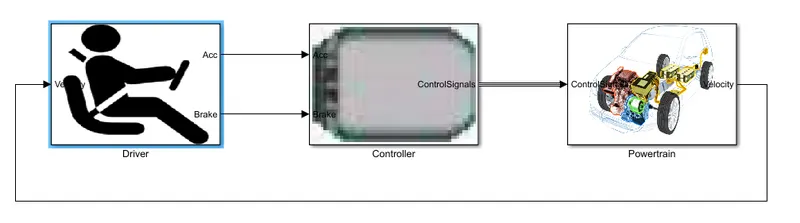
The model used in this project are as follow :

1. Driver Model
2. Controller Model
3. Powertrain Model

Forward Energy-Based Model

1. DRIVER MODEL

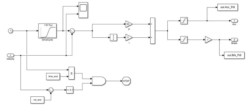
The driver model is used to provide acceleration and brake requirment based on the difference between actual speed of the vehicle and reference speed. The accleration and braking requirement is given by the PI controller for given error. For this model, the proportional gain of 50 and integrator gain of 5 is used as a PI controller constant. Some block is provided for automatically stopping the simulation when time at the drive cycle ends.The figure shown below is the driver block which is used in this project.

2. CONTROLLER MODEL

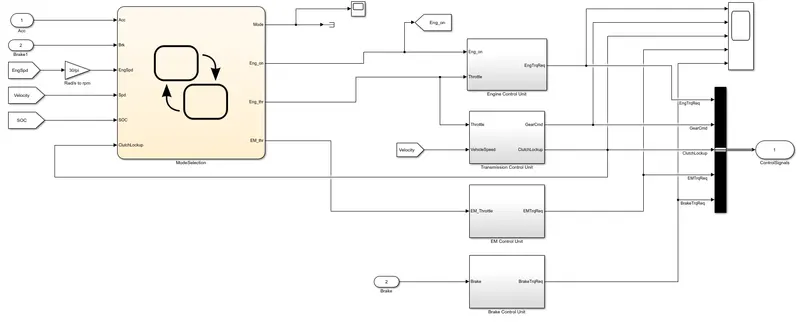
The controller block is performed on different control signal by requesting from the driver block is fed into the controller block. The controller block consists of a master controller(Mode selection), Engine control unit, Transmission Control unit, motor control unit and Brake control unit. From the master control unit different signal is send to the other controller to perform action according to the modes. The figure shown below is the controller block for P1 hybrid model.

2.1. MASTER CONTROLLER(MODE SELECTION)

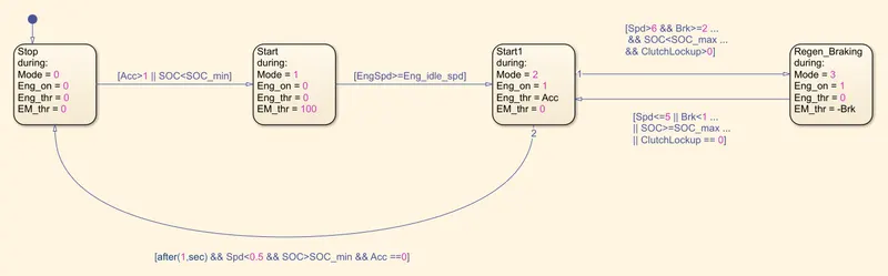
Master control unit is the main control unit for hybrid vehicle.This control unit decides which operation/modes the vehicle should be in. For P1 hybrid two features have been intrgrated i.e. Start and stop and regenerative braking.The figure shown below is the controller logic and based on the input like accleration, braking, engine speed, SOC level, vehicle speed different modes is selected.

2.2 ENGINE CONTROL UNIT

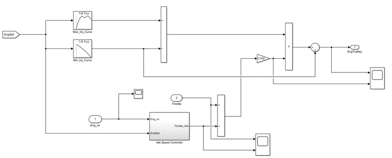
It is based on the engine throttle coming from the master controller, a torque request is supplied to the powertrain blockset. To integrated idle start stop feature, a variable called as engine on is used which value is 0 for engine off and 1 for engine on. The value of engine on is determined by the master controller based on the modes which the vehicle is in. This helps to save fuel when the vehicle is in idling. Figure shown below is an engine control unit used for this project.

2.3 ENGINE TRANSMISSION UNIT

In transmission control unit, based on the throtle request from the master controller and vehicle speed a gear command and clutch lock up command is generated. This command is generated based on the control logic/transmission shift logic define by using the state flow. Figure shown below is the transmission control unit and transmission shift logic.

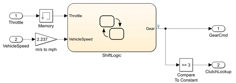
a. transmission control unit

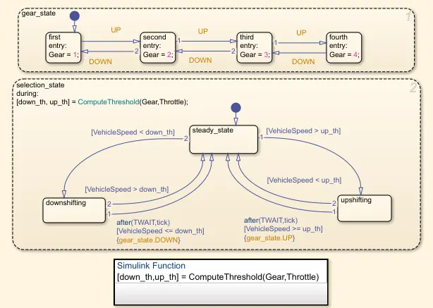
b. transmission shift unit

2.4 MOTOR CONTROL UNIT

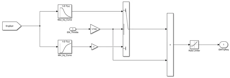
In this control unit, motor throttle request is fed in as a input and based on the speed of motor and throttle , either motoring torque or generating torque is selected from the look up table. This torque is multiplied to get the electric motor torques request. Since the engine is integrated with the electrical machine, the speed of engine is taken as an input speed for a motor. Figure shown below is the Motor control unit that is used in project.

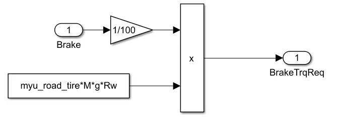
2.5 BRAKE CONTROL UNIT

In this control unit , the braking request from the driver is fetch as an input and based on the braking action of the driver brake torque request is send to the driver. Figure shown below is the brake control unit used in this project.

Now all this control signal from the controller is fetch to the bus creator, which merges the signal and send it to the powertrain block.

3. POWERTRAIN

In powertrain which consists Engine block, Motor block,Transmission block, Differential block, Battery, Wheels and vehicle dynamics block. The control signal from the controller block is send to the powertrain block and based on which the velocity of the vehicle is determined.

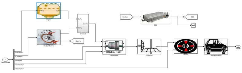
3.1 ENGINE BLOCK

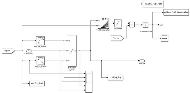
In this block based on the engine speed and torque request from the controller , fuel consumption is taken out by using a lookup table, The torque from the engine is also calculated based on the torque request and engine speed and based on the torque engine speed is also calculated at the transmission block. Figure shown below is the arrangement of simulink block in the engine subsystem.

3.2 MOTOR BLOCK

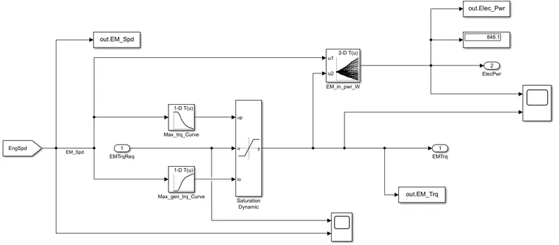
In motor subsystem also, based on the the motor torque request from the controller and engine speed the torque and input power to the motor is calculated. The engine speed is considered because it is considered that engine and motor are running at the same speed in P1 hybrid Vehicle. Figure shown below is the simulink block arrangement for the Motor subsystem.

3.3 TRANSMISSION BLOCK

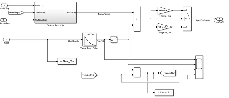
In the transmission subsystem,based on the input crank torque and Transmission In speed,the torque from the torque converter is calculated. Based on the gear command from the controller, gear ratio is selected by considering the gear and gear ratio data from the lookup table. product of gear ratio and torque from the torque converter gives us the total output torque from the transmission. Based on the nature of torque its efficiency is assigned and output torque is calculated. Figure shown below is the block arrangement for the transmission subsystem.

3.4 DIFFERENTIAL BLOCK

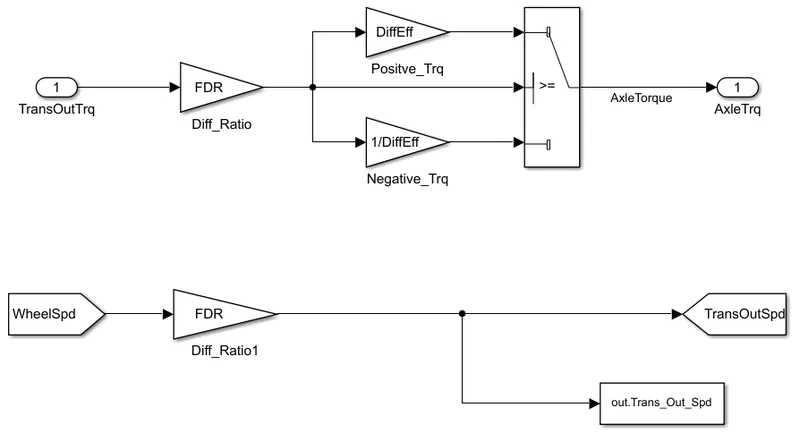
In differential subsystem,transmission output torque is multipled with final drive ratio of the system and based on the nature of the torque, negative or positive axle torque is calculated.

3.5 WHEEL BLOCK

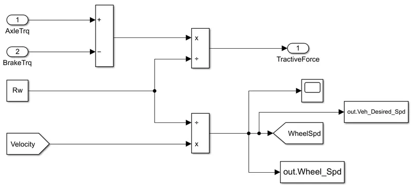
In wheel subsystem, the brake torque request from the brake contoller is fetch in. Based on the brake torque request and axle torque, traction force is calculated by considering the wheel speed. And the traction force is send to the vehicle dynamic subsystem.

3.6 VEHICLE DYNAMICS

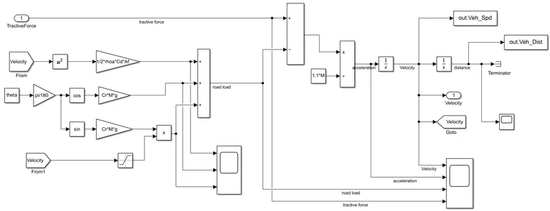
In vehicle dynamic subsystem, all the resistive/ resistance force is calculated.The resistance force is subtracted from the total tractive force and result is divided by the mass of the vehicle to obtain the accleration of a vehicle. The integration of accleration is done to find out the velocity of the vehicle. This velocity is again reverted back to the driver block and based on which driver applies brake or accleration by comparing the velocity with the given drive cycle. Figure shown below is the simulink block arrangement for the Vehicle dynamic subsystem.

3.7 BATTERY MODEL

In battery subsystem,based on the input power demand from the motor, the current from the battery is considered Honda insight motor and battery pack which is takes from NiMH battery pack(5.7, ~6Ah and 148.6V, ~154V). And based on the current drawn , SOC level of the battery is calculated by considered the technique called as columb counting. The Voltage of the battery being the function of the SOC level of the battery, so the open circuit voltage is calculated by SOC level of battery.Figure shown below is the simulink block arrangement for the battery subsystem.

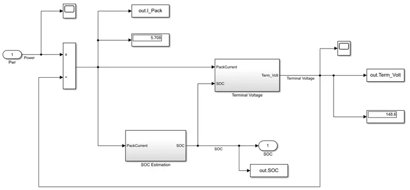
a. Arrangement of ESS (energy storage system)

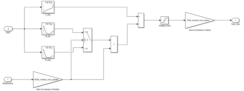
b. Arrangement of Terminal Voltage subsystem

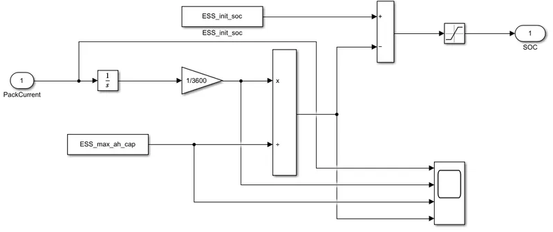
c. Arrangement of SOC(state of charge)

LOGIC AND FORMULA CONSIDERED WHILE MODELING THE P1 HYBRID VEHICLE SYSTEM

FOR CONTROL SUBSYSTEM

a. Logic for master controller

Master controller is developed in such a way that, based on the input to it, vehicle will go to certain mode define by the transition conditions. The Modes considered were Stop , Start, Drive and Braking and based on the modes different value for Engine on condition, Engine throttle ,Motor throttle was given. The transition from one mode to another is given below:

• Stop To Start

Acc>1 || SOC<SOC_min

• Start To Drive

EngSpd>=Eng_idle_spd

• Drive To Braking

Spd>6 && Brk>=2 ...&& SOC0

• Drive To Stop

after(1,sec) && Spd<0.5 && SOC>SOC_min && Acc ==0

• Braking To Drive

Spd<=5 || Brk<1 ...|| SOC>=SOC_max ...|| ClutchLockup == 0

Table 1: Value for Different Variable For each Modes

Modes	Mode	Eng_on	Eng_thr	EM_thr
Stop	0	0	0	0
Start	1	0	0	100
Drive	2	1	Acc	0
Braking	3	1	0	-Brk

b. Engine Controller

Based on the engine speed,From look up table a torque is determined. and that torque is multiplied by acceration request.

• Engine torque = Function(Engine_Speed)
• Engine torque request = Engine torque * Eng_tr * 1/100.

c. Motor Control Unit

Since the engine and motor are considered to be coupled, Based on the engine speed we are determining the torque from the motor. Since the motor can be operated for motoring and generating condition. When the M_tr is positive than motoring torque is considerd and for negative case generating conditions is considered.

• Motor torque = Function(Engine_Speed)
• Motor torque request = M_tr * Motor torque * 1/100

d. Brake Control unit

• Brake Torque = friction coefficient b/w tire and road * Mass of vehicle *acceleration due to gravity * tire radius.

FOR POWERTRAIN SYSTEM

Engine

• Engine Torque=Function(Engine Speed,Eng_troque request)
• Engine_Fuel Consumption=Function(Engine Torque ,Engine Speed)

Motor

• Motor Torque=Function(Engine_Speed,M_torque request)
• Motor Input Power=Function(Engine Speed,Motor Torque)

Key Formulas

• Speed Ratio, S.R = wt/wp
• Torque Ratio, T.R = Tt/Tp
• Capacity factor, K = wp/sqrt(Tp*Wp)
• Road Friction , Fr= Cr*Mg*cos(theta)
• Gradient Force, Fg = Mg*sin(theta)
• Drag force, Fd = 1/2(rho_a*Af*Cd*(Vveh+Vwind)^2)
• Total road load, Fl=Fr+Fg+Fd
• Accleration , a = (Total traction force-Total road load)/M
• velocity, v= integration of (adt)

where,M is the mass of the vehicle, g is the accleration due to gravity, theta is the inclination of road,Af is the frontal area of the vehicle,wt and wp is the speed of the turbine and pump respectively. Tt and Tp is the torque from turbine and pump respectively. rho_a is the density of air.

SCRIPT:

Initally the data for model is loaded by using the Project2_InitFile.m. After running the InitFile.m, go to the simulink model and run the model.After running the simulink model, Now Post processing Script is run. To Know the result for first drive cycle, change the other drive cycle (like UDDS to HWFET etc).

INITIAL MATLAB SCRIPT:

%%%%%%%%%%%%%%%%%%%%%%%%%%%%%%%%%%%%%%%%%%%%%%%%%%%%%%%%%%%%%%%%%%%%%
%% Skill-Lync -> Development of Hybrid Drives
% Project - Hybrid Vehicle Model

% Description:

%% Initialization File
% Initialization file for loading the variables for the Conventional vehicle simulation model

clear all
close all
clc

%% Vehicle Parameters
M = 1500; % Vehicle weight [kg]
Cr = 0.015; % Rolling resistance coefficient
Rw = 0.35; % Rolling radius [m]
Cd = 0.33; % Drag coefficient
Af = 2; % Frontal area [m2]
rhoa = 1.225; % Air density [kg/m3]
Vwind = 0; % Wind velocity [kmph]
g = 9.81; % Gravitational acceleration [m/s2]
theta = 0; % Slope [deg]
myu_road_tire = 1; % Coefficient of friction between tire - road interface

%% Powertrain Parameters
FDR = 3.73; % Final Drive Ratio / Diff Ratio
DiffEff = 0.99; % Differential efficiency (assumed independent of operating conditions)

NumGear = 4; % Number of gears in transmission
TransGear = [1:NumGear]; % Transmission Gears
TransRatio = [3.06, 1.62, 1, 0.7]; % Corresponding Transmission ratios
TransEff = 0.90; % Transmission efficiency (assumed independent of operating conditions)

TC_SR = [0, .5, .6, .7, .8, .87, .92, .94, .96, .97, 1]; % Torque Converter Speed Ratio (Matlab default) -> TurbSpd/PumpSpd
TC_TR = [2.232, 1.5462, 1.4058, 1.2746, 1.1528, 1.0732, 1.0192, 1, 1, 1, 1]; % Torque Converter Torque Ratio (Matlab default) -> TurbTrq/PumpTrq
TC_Cf = 1e-4 * [.72558, .66322, .63463, .59042, .51331, .4144, .29287, .22444, .12186, .04386, 0]; % Torque Converter Capacity Factor (Matlab default) -> PumpTrq/PumpSpd^2 [Nm/rpm^2]

load Vehicle_Data/Engine_data_1_9L_Saturn_95kW
load Vehicle_Data/Trans_Shift_map
load Vehicle_Data/EM_Honda_Insight_10kW
load Vehicle_Data/ESS_NiMH6
load Vehicle_Data/EM_Westinghouse_75kW_AC_induction.mat
load Vehicle_Data/Torque_Converter_data.mat

ESS_init_soc = 0.8;
ESS_soc_max = 0.9;
ESS_soc_min = 0.6;

%% Driver Parameters
Kp = 10; % P gain for driver PI model
Ki = 1; % I gain for driver PI model
Drive_Cycle_Select = 1; % Drive cycle selection

% Drive cycle values in m/s

if Drive_Cycle_Select == 1
load DriveCycles/UDDS;

elseif Drive_Cycle_Select == 2
load DriveCycles/HWFET;

elseif Drive_Cycle_Select == 3
load DriveCycles/FTP;

elseif Drive_Cycle_Select == 4
load DriveCycles/US06;

elseif Drive_Cycle_Select == 5
load DriveCycles/NEDC;

elseif Drive_Cycle_Select == 6
load DriveCycles/WLTP;

end

time_end = cyc_time(end);
vel_end = cyc_vel(end);

POST PROCESSING SCRIPT:

%%%%%%%%%%%%%%%%%%%%%%%%%%%%%%%%%%%%%%%%%%%%%%%%%%%%%%%%%%%%%%%%%%%%%
%% Skill-Lync -> Development of Hybrid Drives
% Project - Hybrid Vehicle Model
% By - Vikash Kumar

% Description:
% The following file is to used with the Initialization file and Simulink
% results for post-processing of the data.
% The file is incomplete, has some examples of how the data is imported
% into a readable format, data analysis and plotting examples.
% Based on the project task, use commands in a similar format as given
% below, to analyse the data and generate required plots.
% You can change variable names if desired

%% Post-Processing File
% File for post-processing the Conventional vehicle simulation model data

close all

%% Renaming variables
Time = out.tout;
Acc_Pdl = out.Acc_Pdl; % Accelerator pedal [%]
Brk_Pdl = out.Brk_Pdl; % Brake pedal [%]
Gear_Cmd = out.Gear_Cmd; % Transmission gear
Trans_In_Spd = out.Trans_In_Spd*30/pi; % Transmission input speed [rpm]
Trans_Out_Spd = out.Trans_Out_Spd*30/pi; % Transmission output speed [rpm]
Eng_Trq = out.Eng_Trq; % Engine brake torque [Nm]
Eng_Spd = out.Eng_Spd*30/pi; % Engine speed [rpm]
Eng_Fuel_Consump = out.Eng_Fuel_Consumption; % Engine fuel consumption [g]
Veh_Dist = out.Veh_Dist/1000; % Distance traveled by vehicle [km]
Veh_Spd = out.Veh_Spd*18/5; % Vehicle speed [kmph]
Wheel_Spd = out.Wheel_Spd*30/pi; % wheel speed [rpm]
Eng_Fuel_Rate = out.Eng_Fuel_Rate; % Engine fuel flow rate [%]
Veh_Desired_Spd = out.Veh_Desired_Spd; % vehicle desired speed [kmph]
% electric machine
EM_Spd = out.EM_Spd; % Electric motor speed [rpm]
EM_Trq = out.EM_Trq; % Electric motor torque [N-m]
Elec_Pwr = out.Elec_Pwr; % Electric motor power [KW]
% ESS - energy storage system
packcurrent = out.I_Pack; % Pack current [Ah]
term_volt = out.Term_Volt; % Terminal voltage [V]
SOC = out.SOC; % state of charge [%]

%% Data Analysis
Eng_Pwr = Eng_Spd*pi/30.*Eng_Trq/1000; % Engine brake power [kW]
rho_petrol = 0.7197; % Density of petrol [kg/L]
kmpl = Veh_Dist(end)/(Eng_Fuel_Consump(end)/1000/rho_petrol); % Fuel economy [kmpl]

% T_dis = Veh_Dist(end); % total distance in km
% T_fuel = Eng_Fuel_Consump(end); % total fuel consume
% Volume = (T_fuel/1000)/rho_petrol; % total litre of fuel
% Milage = T_dis/Volume; % milage in kmpl

%% Plotting vehicle characteristics time trace Engine speed,Transmission I/P spd, Transmission O/P Spd and Wheel Speed
figure(1)
hold on
grid on
plot(Time,Eng_Spd,'LineWidth',1,'Color','g');
plot(Time,Trans_In_Spd,'LineWidth',1,'Color','black');
plot(Time,Trans_Out_Spd,'LineWidth',1,'Color','red');
plot(Time,Wheel_Spd,'LineWidth',1,'Color','blue');

xlabel('Time [s]')
ylabel('Speed [rpm]')
xlim([0, Time(end)]);
ylim([0, 6000]);
legend('Engine Speed','Transmission I/P Spd','Transmission O/P Spd','Wheel Speed');

%% Plotting vehicle characteristics time trace engine torque, engine power, fuel rate and fuel consumption

figure(2)
subplot(2,2,1)
plot(Time,Eng_Trq,'LineWidth',1,'Color','g')
xlabel('Time [s]')
ylabel('Torque [Nm]')
legend('Torque')

subplot(2,2,2)
plot(Time,Eng_Pwr,'LineWidth',1,'Color','black')
xlabel('Time [s]')
ylabel('Power [kW]')
legend('Engine Power')

subplot(2,2,3)
plot(Time,Eng_Fuel_Rate,'LineWidth',1,'Color','red')
xlabel('Time [s]')
ylabel('Fuel Rate [%]')
legend('Fuel Flow Rate')

subplot(2,2,4)
plot(Time,Eng_Fuel_Consump,'LineWidth',1,'Color','blue')
xlabel('Time [s]')
ylabel('Fuel Consumption [kmpl]')
legend('Fuel Consumption')

%% Plotting vehicle characteristics time trace accelerator and brake pedal, gear command, vehicle desired,distance travelled and actual speed .
figure(3)
subplot(2,2,1)
hold on
grid on
plot(Time, Acc_Pdl, 'linewidth', 1, 'Color', 'black');
plot(Time, Brk_Pdl, 'linewidth', 1, 'Color', 'red');
ylabel('Pedal [%]')
xlim([0, Time(end)]);
legend('Acc','Brake');
subplot(2,2,2)
hold on
grid on
plot(Time,Veh_Spd, 'linewidth', 1, 'Color', 'black');
plot(Time,Veh_Desired_Spd, 'linewidth', 1, 'Color', 'red');
ylabel('Speed [rpm]')
xlim([0, Time(end)]);
legend('Vehicle Actual Speed','Vehicle Desired Speed');
subplot(2,2,3)
hold on
grid on
plot(Time, Gear_Cmd, 'linewidth', 1, 'Color', 'black');
xlim([0, Time(end)]);
xlabel('Time [s]');
ylabel('Gear');
title('Gear command')
subplot(2,2,4)
hold on
grid on
plot(Time, Veh_Dist, 'linewidth', 1, 'Color', 'black');
xlim([0, Time(end)]);
xlabel('Time [s]');
ylabel('Distance [km]');
title('Distance Travelled')

%% Plotting engine operating points on engine fuel map
figure('Name','Engine Operating Points');
hold on
grid on
title('Engine Operating Points','fontsize',12);
p1=plot(Eng_map_spd*30/pi,Eng_max_trq,'linewidth',2,'color','r');
p2=line([Eng_map_spd(end)*30/pi Eng_map_spd(end)*30/pi],[0 Eng_max_trq(end)]);
set(p2,'linewidth',1,'linestyle','--','color','k');
p3=line([Eng_map_spd(1)*30/pi Eng_map_spd(1)*30/pi],[0 Eng_max_trq(1)]);
set(p3,'linewidth',1,'linestyle','--','color','k');
[c,h] = contour(Eng_map_spd'*30/pi,Eng_map_trq,Eng_fuel_map');
clabel(c,h);
xlabel('Engine Speed [rpm]');
ylabel('Engine Torque [Nm]');
title('Engine Fuel Consumption Map [g/s]');
p4 = plot(Eng_Spd,Eng_Trq,'.','color','k');
legend([p1 p4],{'Max Curve','Operating Points'});
axis([Eng_map_spd(1)*30/pi Eng_map_spd(end)*30/pi 0 Eng_map_trq(end)]);

%% Plotting vehicle characteristics time trace motor speed, motor torqe and motor power
figure(5)
subplot(2,2,1)
hold on
grid on
plot(Time,EM_Trq,'LineWidth',1,'Color','g')
xlabel('Time [s]')
ylabel('Torque [Nm]')
legend('Motor Torque')

subplot(2,2,2)
hold on
grid on
plot(Time,EM_Spd,'LineWidth',1,'Color','g')
xlabel('Time [s]')
ylabel('Speed')
legend('Motor Speed')

subplot(2,2,3)
hold on
grid on
plot(Time,Elec_Pwr,'LineWidth',1,'Color','black')
xlabel('Time [s]')
ylabel('Power [kW]')
legend('Motor Power')

%% Plotting graph between time vs current, terminal voltage and state of charge
figure(6)
subplot(2,2,1)
hold on
grid on
plot(Time,term_volt,'r');
xlabel('Time');
ylabel('Terminal Voltage [V]');
title('Terminal Voltage plot');
subplot(2,2,2)
hold on
grid on
plot(Time,SOC,'g');
xlabel('Time');
ylabel('SOC');
title('State Of Charge [%]');
subplot(2,2,3)
hold on
grid on
plot(Time,packcurrent,'b');
xlabel('Time');
ylabel('Current in Amp');
title('Pack Current');

%% Plotting motor operating points on engine fuel map

figure('Name','Motor Operating Points');
hold on
title('Motor Operating Points','fontsize',12)
plot(EM_map_spd*30/pi,EM_max_trq,'linewidth',2,'color','b','Displayname','Maximum Torque');
plot(EM_map_spd*30/pi,EM_max_gen_trq,'linewidth',2,'color','r','Displayname','Maximum Generating Torque')
plot(EM_Spd*30/pi,EM_Trq,'.','color','k','Displayname','Operating Point');
contour(EM_map_spd'*30/pi,EM_map_trq,EM_eff_map','ShowText','on','Displayname','Efficiency');
legend
hold off
grid off

Based on the need of the cycle, the cycle is selected from the initialization script. For UDDS cycle , we have selected the Drive cycle as 1 and for HWFET we have to select it as 2.

PLOT OBTAINED FROM MATLAB

The model had been run for the different cycle and different parameters were analysised and compared with the conventional vehicle model.

Comparision for Different Drive Cycle

Two drive cycle UDDS and HWFET were considered and different system level parameters were analysised.

Comparision for Speed for engine,wheel and Transmission for both Drive cycle.

Figure (a) shows the speed of the engine,wheel and transmission system for UDDS cycle while the figure (b) shows the same for the HWFET cycle. In the UDDS cycle we can observe the average speed of the wheel transmission and engine is higher in case of the HWFET cycle as the vehicle has to propel with higher velocity as compared with UDDS cycle. It was also observed that in UDDS cycle, there is frequent rise and fall in the speed of the wheel, engine and transmission than HWFET cycle. This is due to the frequent stop start condition in urban driving condition.

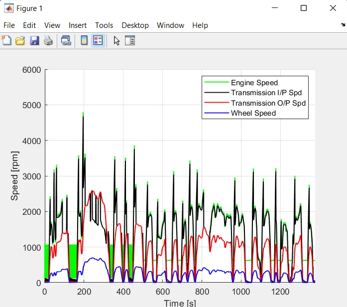
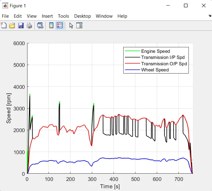
(a) Speed for different component for UDDS cycle (b) Speed for different component for HWFET cycle

Engine power,torque, flow rate and fuel consumption Analysis for HWFET cycle and UDDS cycle

In UDDS cycle, we can observe that,there is frequent rise and fall in engine power and torque while for HWFET cycle, the fall and rise is compartively smaller than the UDDS cycle as shown in the figure a and b. This enables the HWFET cycle to work in the more efficient region as shown in figure as compared with UDDS cycle which lower the fuel consumption rate. The highest fuel consumption rate for UDDS cycle is around 4 gm/sec, while for HWFET cycle it is around 3.2 gm/sec.In HWFET cycle the works more in a higher efficient region when compared with the UDDS cycle. In HWFET cycle we can observe the minimum amount of negative torque from the engine when compared with UDDS cycle, as in highway vehicle do not have to deal with frequent start stop condition. At the end of the drive cycle,the overall consumption of the was around 700 gm for HWFET cycle and around 600 gm for UDDS cycle.

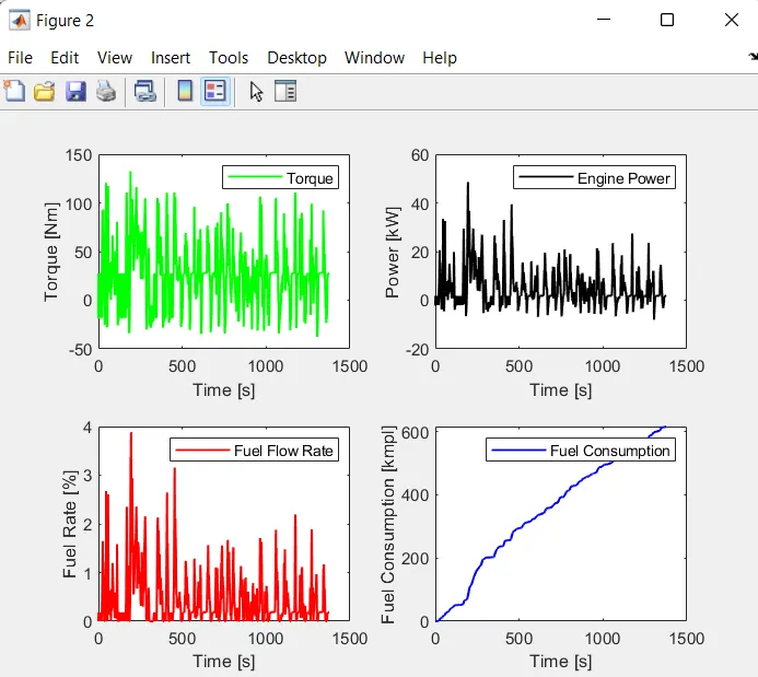
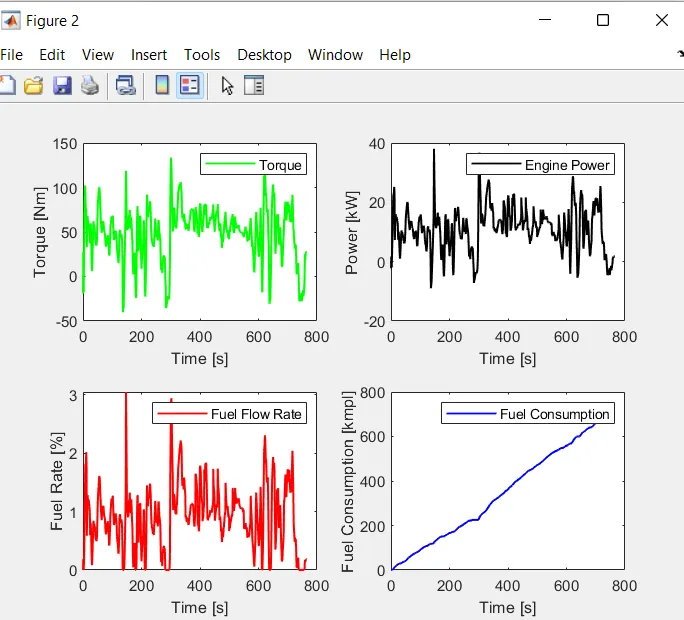
(a) Engine power/torque and fuel consump. for UDDS cycle (b) Engine power/toque and fual consump. for HWFET cycle

Acclerator, Brake pedal position and Gear Selected for different drive cycle and also distance travelled

Figure (a) shows the brake pedal and accelerator pedal position for UDDS cycle.We can observe that when the vehicle is following the UDDS cycle the use of the brake pedal is quite often and the intensity for the pedal is pressed is also high as compared with the HWFET cycle in figure (b). The vehicle is often in a higher gear for the HWFET cycle as compared with the UDDS cycle. The vehicle has cover the distance of around 12 km for the UDDS cycle and around 17km for HWFET cycle.

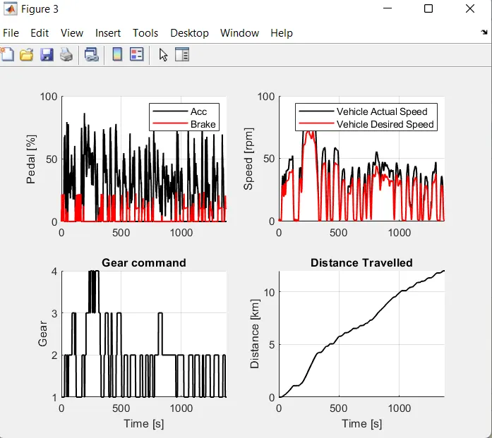
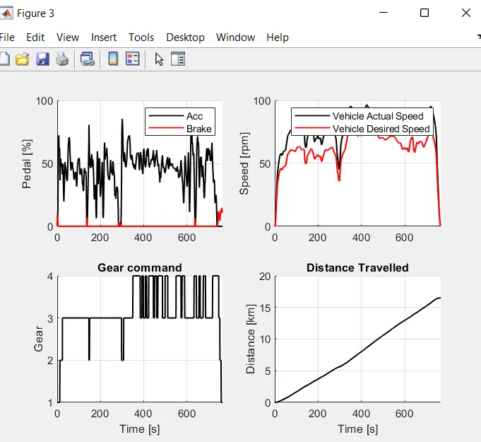
(a) Accelerator, Brake peddle position and gear command for UDDS (b)Accelerator, Brake peddle position and gear command for HWFET cycle

Comparision for motor speed , torque and input power for both UDDS and HWFET cycle

Figure shows the motor power , torque and speed for UDDS cycle and also for HWFET cycle.We can observe that when the vehicle is following the UDDS cycle torque is more compare to HWFET but motor speed in HWFET is more as well as motor power throught the cycle.

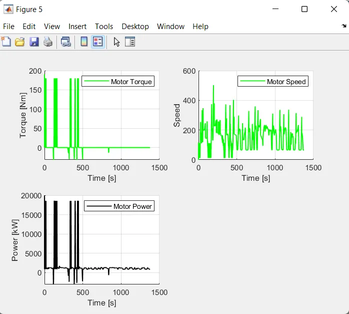
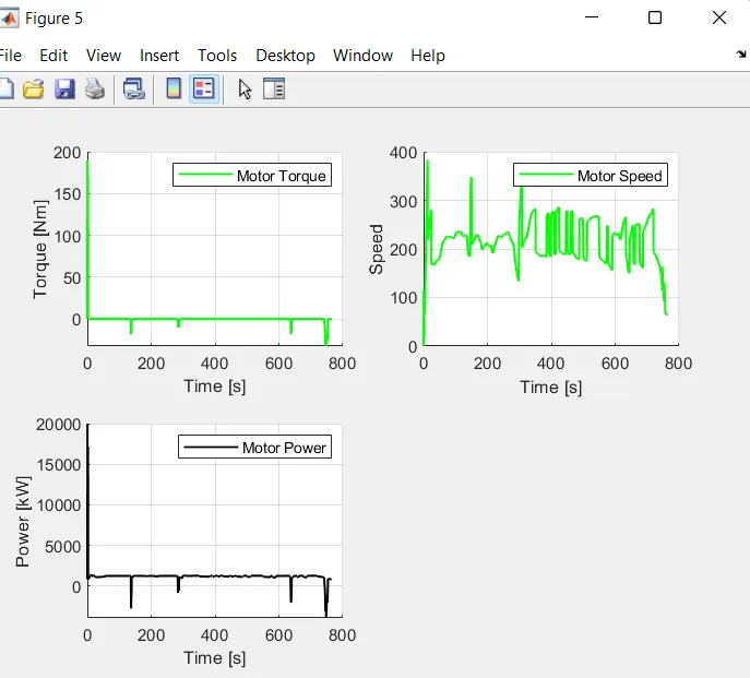
(a) Motor speed, torque and input power for UDDS cycle (b) Motor speed, torque and input power for HWFET cycle.

Comparision between pack current, voltage and state of charge for both the UDDS and HWFET cycle

In UDDS cycle, there is a frequent fall in terminal voltage but in figure b, terminal voltage quite constant with time, but at same time we seen packcurrent quite rise and fall in UDDS but in HWFET, firsst initialise and rest is almost constant throughout whole time. SOC in UDDS cycle tend to almost 1400 s but in HWFET cycle tend to 700 s.

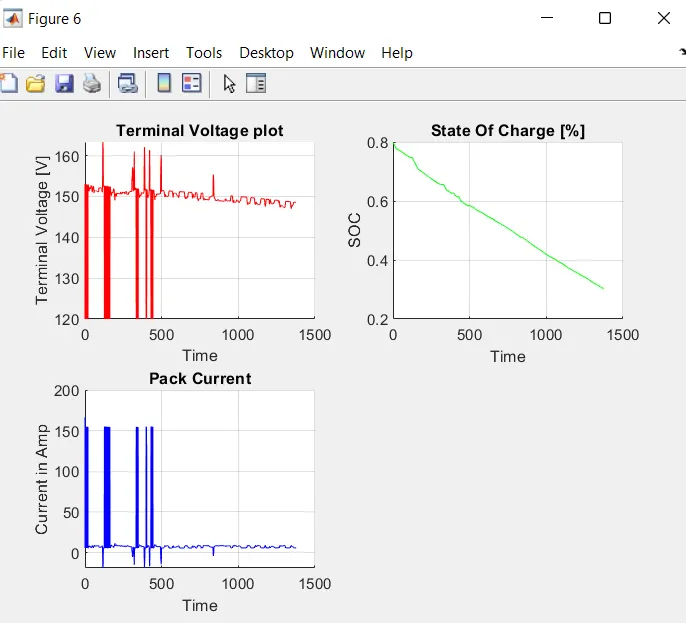
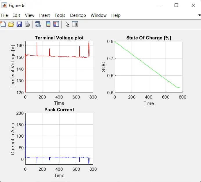
(a) Packcurrent, voltage and SOC for UDDS cycle (b) Packcurrent, voltage and SOC for HWFET cycle.

Motor operating point for both the UDDS and HWFET cycle

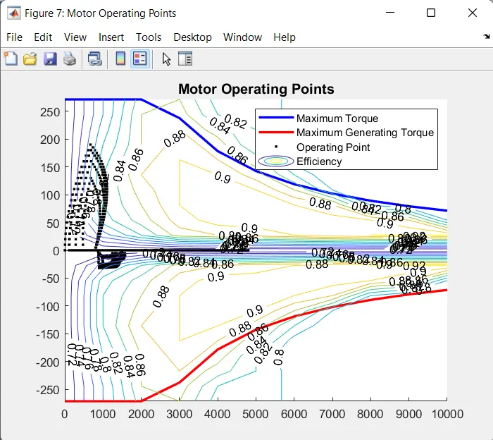
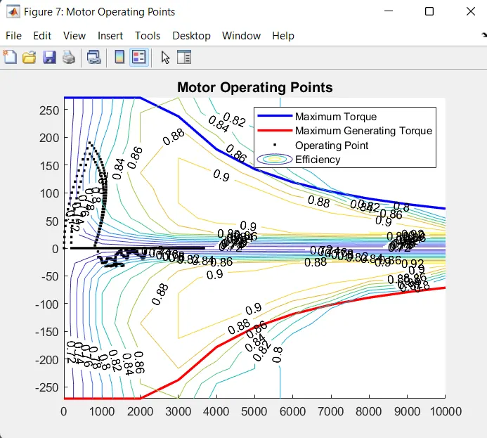
Motor Operating Point for both the cycle

Comparision inbetween Hybrid vehicle and Conventional Vehicle

Figure (a) is the engine fuel consumption map with its operating point when we have considered the hybrid vehicle and figure(b) is the engine fuel consumption plot with itsoperating point when we have considered the conventional vehicle for UDDS cycle.We can oberve comparitively large amount of cluster of operating point for conventional vehicle than for hybrid vehicle. This is due to the start stop feature in the hybrid vehicle which stops the engine when it is idealing. In figure (a) and (b) is the engine fuel consumption for the HWFET cycle for hybrid vehicle and conventional vehicle. There is some better in terms of the fuel consumption since the HWFET cycle is not subjected to frequent start and stop so similar kind of operating region were observed for the HWFET cycle. The milage for the conventional vehicle when UDDS cycle was considered was around 13.6212 kmpl and for hybrid it was slightly better with 14.0036 kmpl.For HWFET cycle, the milage was increased to 16.9689 kmpl for hybrid vehicle as compared with 16.3072 kmpl for the conventional vehicle. Since, the applied hybrid vehicle was only capable for the start stop and regenerative braking ,milage can be further increase when P2,P3 or above model were considered in which more features like motor assist or EV alone mode is also available.

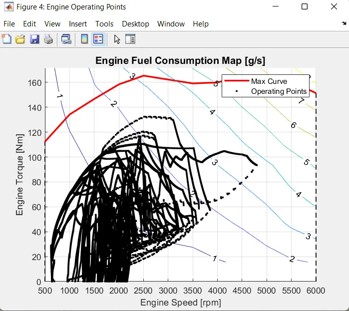
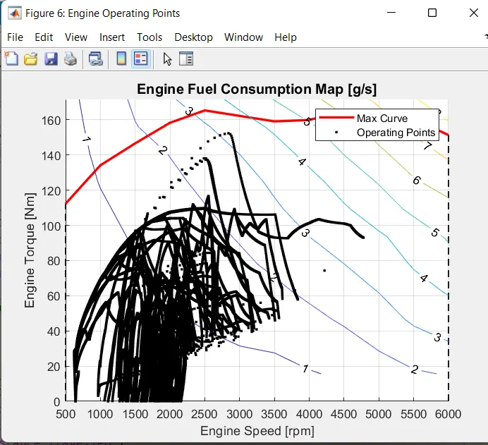
(a)Engine performance map with its operating point for hybrid vehicle in UDDS cycle. (b)Engine perfromace map with its operating point for conventional vehicle in UDDS cycle.

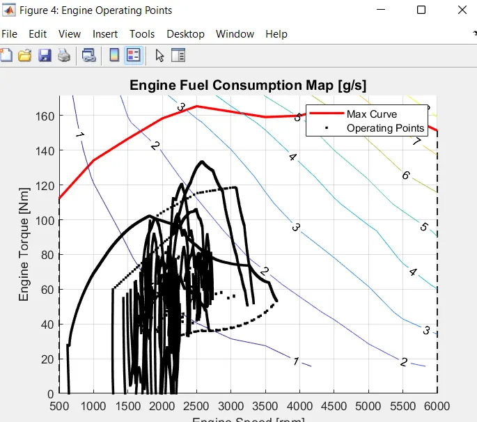
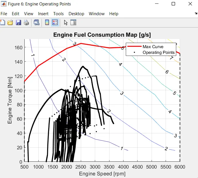
(a)Engine performance map with its operating point for hybrid vehicle in HWFET cycle. (b)Engine perfromace map with its operating point for conventional vehicle in HWFET cycle.

Conclusion:

The system level analysis is done for the P1 hybrid vehicle and compared the fuel consumption aspect or milage with the conventional vehicle.