Week 5 - Curve fitting

AIM :

To write a program in python for curve fit.

Objectives :

1. What does popt and pcov mean?

2. What does np.array(temperature) do?

3. What does the * in *popt mean?

4. Write code to fit a linear and cubic polynomial for the Cp data. Explain if your results are good or bad.

5. What needs to be done in order to make the curve fit perfect?

6. Show empirically as to how well your curve has been fit.

Theory:

Curve fitting is the process of constructing a curve, or mathematical function, that has the best fit to a series of data points, possibly subject to constraints. Curve fitting can involve either interpolation, where an exact fit to the data is required, or smoothing, in which a "smooth" function is constructed that approximately fits the data. A related topic is regression analysis, which focuses more on questions of statistical inference such as how much uncertainty is present in a curve that is fit to data observed with random errors. Fitted curves can be used as an aid for data visualization, to infer values of a function where no data are available, and to summarize the relationships among two or more variables.

Linear, Polynomial, and Multiple Regression

Linear and Polynomial regressions in Origin make use of the weighted least-square method to fit a linear model function or a polynomial model function to data, respectively.

Linear Fit

Masking outliers during linear fit

Linear fit with fixed intercept or slope

Ellipse Plot for graphical examination of linearity

Linear Fit with X Error PRO

Apparent Fit

Polynomial Fit

The Polynomial Fit tool in Origin can fit data with polynomial up to 9th order. Fixed intercept and apparent fit are also supported.

Multiple Linear Regression

Multiple Linear Regression fits multiple independent variables

A unique feature of Origin's Multiple Linear Regression is Partial Leverage Plots, useful in studying the relationship between the independent variable and a given dependent variable:

Type of curve fitting including:

• Interpolation, Where you discover a function that is exact to the data points. Since this assumes no measurement error, it has limited application to real-life scenarios.
• Smoothing is when we find a function that is an approximate fit to the data points, but we give room for error and we allow our actual points to be near, but not necessarily on the line; given the error is minimized overall.

THE CODE:

import math
import matplotlib.pyplot as plt
import numpy as np
from scipy.optimize import curve_fit

#linear fit
def func(t,a,b,c):
	return a*pow(t,2) + b*t + c

#cubic fit
def func1(t,a,b,c,d):
	return a*pow(t,3) + b*pow(t,2) + c*t + d

# reading thermodinamic data files
def read_file():
	tempreature = []
	cp = []
	for line in open('data','r'):
		value = line.split(',')
		tempreature.append(float(value[0]))
		cp.append(float(value[1]))
		
	return [tempreature,cp]

#linear fit
tempreature,cp = read_file()
popt,pcov = curve_fit(func,tempreature,cp)
fit_cp = func(np.array(tempreature),*popt)

plt.plot(tempreature,cp,'k--')
plt.plot(tempreature,fit_cp,color='red')
plt.legend(['Actual data','curve fit'])
plt.xlabel('tempreature(k)')
plt.ylabel('cp')
plt.title('cubic curve fitting')
plt.show()

#Cubic fit
popt,pcov = curve_fit(func1,tempreature,cp)
fit_cp = func1(np.array(tempreature),*popt)

plt.plot(tempreature,cp,'k-')
plt.plot(tempreature,fit_cp,color='red')
plt.legend(['Actual data','curve fit'])
plt.xlabel('tempreature(k)')
plt.ylabel('cp')
plt.title('cubic curve fitting')
plt.show()

THE STEPS :

First, we import all the essential modules needed for the code to run.

Then we call for functions that govern linear and cubic equations

The following data is loaded into Python by placing it in the right directory and a function read_file is created. For loop is used to run each line by using the 'open' command with 'r' to read it.

from the data, we extract temperature and cp values

For curve fitting, 'popt' and 'pcov' are used as output fostoring parameters obtained by 'curve_fit' command which takes input as the required function(linear or cubic) , temperature, and Cp. Now, another variable named 'fit_cp' stores the new values of Cp calculated by using temperature array.

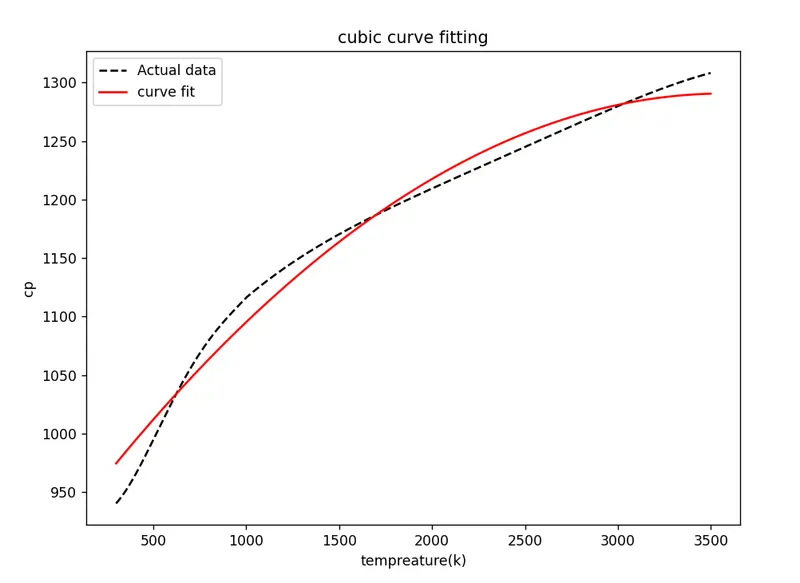
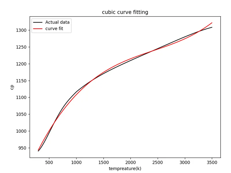
Plots of both raw dataset and predicted dataset are made and compared to find fitness characteristics for both the curves for both linear and cubic polynomial.

The Results:

1. What do popt and pcov mean?

popt- An array of optimal values for the parameters which minimize the sum of squares of residuals.

The returned parameter covariance matrix pcov is based on scaling sigma by a constant factor. This constant is set by demanding that the reduced chisq for the optimal parameters popt when using the scaled sigma equals unity. In other words, sigma is scaled to match the sample variance of the residuals after the fit.

2. What does np.array(temperature) do?

NumPy arrays facilitate advanced mathematical and other types of operations on large numbers of data. Typically, such operations are executed more efficiently and with less code than is possible using Python's built-in sequences.

3.What does the * in *popt mean?

'*' , '*popt' indicates and returns each coefficient stored in popt array.

4.Write code to fit a linear and cubic polynomial for the Cp data. Explain if your results are good or bad.

The code is already written and explained above .By observation it is noted that the increase in degree of polynomial gives us the prefect curve fit. Thus in the given problem cubic curves can be made as best fits.

5,What needs to be done in order to make the curve fit perfect?

If we increase the order of the polynomial, the error produced will be less and curve fit perfectly. On increasing the order of the polynomial the value of will be close to 1 and is assumed to a perfect fit.

6.Show empirically as to how well your curve has been fit.

By observation, a cubic predicted curve has been almost fit into original data curve with some tolerance compared to linear predicted curve.