Week 5 - Curve fitting

Objective : To perform curve fitting.

Program:

# Curve Fitting

import math 
import matplotlib.pyplot as plt 
import numpy as np 
from scipy.optimize import curve_fit 
 
# Curve fitting functions
# Linear function 

def function_1(t,a,b):  
	return a*t + b  

# Cubic function 

def function_2(t,a,b,c,d):  
	return a*pow(t,3) + b*pow(t,2) + c*t +d   
 
# Reading thermodynamic data file 

def read_file():  
	temperature = []  
	cp = []  
	for line in open('data','r'):   
		values = line.split(',')   
		temperature.append(float(values[0]))   
		cp.append(float(values[1])) 
 
	return [temperature, cp] 

 
# Storing temperature and cp in the form of lists
temperature, cp = read_file() 
 
popt, pcov = curve_fit(function_1,temperature,cp) 
fit_cp_l = function_1(np.array(temperature), *popt) 

# For Linear curve fit 

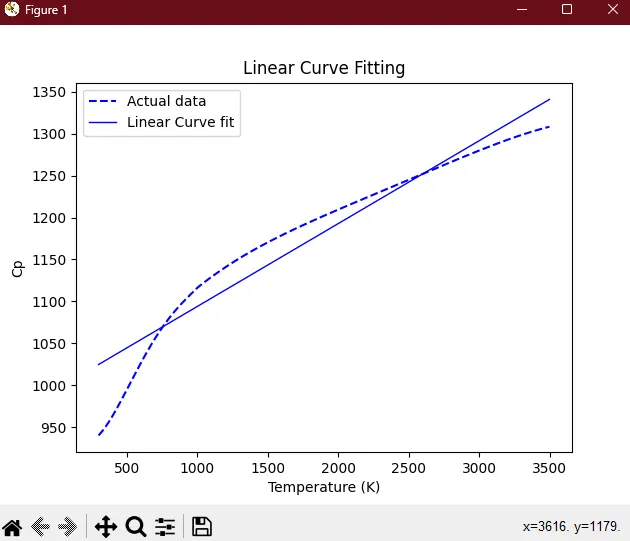
print('For Linear Fit') 
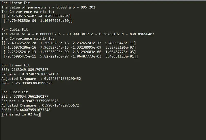
print('The value of parametrs a = ' + '%.3f' %(popt[0]) + ' & b = ' + '%.3f' %(popt[1]))  
print('The Co-varience matrix is:' + '\n' + str(pcov)) 

# Linear curve fit plot

plt.figure(1) 
plt.plot(temperature,cp,'b--') 
plt.plot(temperature,fit_cp_l,color='blue',linewidth = 1) 
plt.legend(['Actual data','Linear Curve fit']) 
plt.xlabel('Temperature (K)') 
plt.ylabel('Cp') 
plt.title('Linear Curve Fitting') 
plt.show() 


popt, pcov = curve_fit(function_2,temperature,cp) 
fit_cp_c = function_2(np.array(temperature), *popt) 

# For Cubic curve fit 

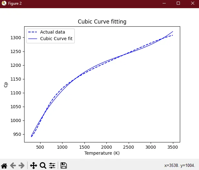
print('\nFor Cubic Fit:') 
print('The value of a = ' + '%.8f' %popt[0] + ' b = ' + '%.8f' %popt[1] + ' c = ' + '%.8f' %popt[2] + ' d = ' + '%.8f' %popt[3]) 
print('The Co-varience matrix is: \n' + str(pcov))

# Cubic curve fit plot

plt.figure(2) 
plt.plot(temperature,cp,'b--') 
plt.plot(temperature,fit_cp_c,color='blue',linewidth = 1) 
plt.legend(['Actual data','Cubic Curve fit']) 
plt.xlabel('Temperature (K)') 
plt.ylabel('Cp') 
plt.title('Cubic Curve fitting') 
plt.show() 
 
 
"""
 Measuring the fitness characetristics of the curves  
 
1. Sum of squares due to error (SSE)
SSR (sum of squares of the regression)  
SST = SSE + SSR

2. R-square 

3. Adjusted R-square

4. Root mean squared error (RMSE) 

 Finding mean of Cp data  
 mean = ( sum of all elements)/(total number of elements)

 """ 
 
s = np.sum(cp) 
l = np.size(cp) 
m = s/l 

# For Linear curve fit 

print('\nFor Linear Fit') 

linear_ssr = 0 
linear_sse = 0 

for i in range(l):     
	linear_error = abs((np.sum((cp[i] - fit_cp_l[i]))))     
	linear_sse = linear_sse+pow(linear_error,2)  						# Sum of squared errors   
	linear_ssr = linear_ssr+ np.sum(pow((fit_cp_l[i] - m),2)) 			# Sum of squares of regression


print('SSE:',linear_sse) 

linear_sst = linear_sse + linear_ssr		               # Total of sum of squares

# Calculating R-square

linear_Rsquare = linear_ssr/linear_sst 
print('Rsquare :' ,linear_Rsquare)

# Calculating Adjusted R-square

k=1;                                                      # No. of independent variables 
AdRsquare_L = 1- (((1-linear_Rsquare)*(l-1))/(l-k-1));    # For linear fit 
print('Adjusted R-square  :' ,AdRsquare_L)

# Calculating Root mean squared error (RMSE)

linear_rmse = pow((linear_sse/l),0.5) 
print('RMSE :',linear_rmse) 
print('') 
 
 
# For Cubic curve fit

print('For Cubic Fit') 

cubic_sse = 0 
cubic_ssr = 0 

for j in range(l):     
	cubic_error = abs(np.sum((cp[i] - fit_cp_c[i])))     
	cubic_sse = cubic_sse+(pow(cubic_error,2))    					# Sum of squared errors  
	cubic_ssr = cubic_ssr+np.sum(pow((fit_cp_c[i] - m),2)) 			# Sum of squares of regression
 

print('SSE :',cubic_sse) 
 
cubic_sst = cubic_sse + cubic_ssr 		                            # Total of sum of squares

# Calculating R-square

Cubic_Rsquare= cubic_ssr/cubic_sst 
print('Rsquare :',Cubic_Rsquare) 

# Calculating Adjusted R-square  

AdRsquare_C = 1- (((1-Cubic_Rsquare)*(l-1))/(l-k-1));              # Adjusted r square for cubic fit
print('Adjusted R-square :' ,AdRsquare_C)

# Calculating Root mean squared error (RMSE) 

cubic_rmse = pow((cubic_sse/l),0.5) 
print('RMSE:',cubic_rmse)

Output:

Split wise fitting of cubic curve:

# Cubic fit

import math 
import matplotlib.pyplot as plt 
import numpy as np 
from scipy.optimize import curve_fit 
 
# Curve fitting functions

# Cubic function  

def function_1(t,a,b,c,d):  
	return a*pow(t,3) + b*pow(t,2) + c*t +d   
 
# Reading thermodynamic data file 

def read_file(): 
	temperature = []  
	cp = []  
	for line in open('data','r'):   
		values = line.split(',')   
		temperature.append(float(values[0]))   
		cp.append(float(values[1])) 
 
	return [temperature , cp] 

temperature = []  
cp = []  
 
# Storing temperature & cp in the form of lists

temperature , cp = read_file() 

# Split the data into 5 parts
 
temperature1 = temperature[1:640];
cp1 = cp[1:640];

temperature2=temperature[641:1280];  
cp2 = cp[641:1280]; 
 
temperature3=temperature[1281:1920];  
cp3 = cp[1281:1920];   

temperature4=temperature[1921:2560];  
cp4 = cp[1921:2560];  
 
temperature5=temperature[2561:3200]; 
cp5 = cp[2561:3200]; 


# Cp=a*t^3+b*t^2+ct+d  
popt, pcov = curve_fit(function_1,temperature1,cp1) 
fit_cp_l = function_1(np.array(temperature1), *popt) 

popt, pcov = curve_fit(function_1,temperature2,cp2) 
fit_cp_2 = function_1(np.array(temperature2), *popt) 

popt, pcov = curve_fit(function_1,temperature3,cp3) 
fit_cp_3 = function_1(np.array(temperature3), *popt) 

popt, pcov = curve_fit(function_1,temperature4,cp4) 
fit_cp_4 = function_1(np.array(temperature4), *popt) 

popt, pcov = curve_fit(function_1,temperature5,cp5) 
fit_cp_5 = function_1(np.array(temperature5), *popt) 



# Split curve fit Plot

plt.figure(1) 
plt.plot(temperature,cp,'y',linewidth = 4 ) 
plt.plot(temperature1,fit_cp_l,'k--',linewidth = 1) 
plt.plot(temperature2,fit_cp_2,'k--',linewidth = 1) 
plt.plot(temperature3,fit_cp_3,'k--',linewidth = 1) 
plt.plot(temperature4,fit_cp_4,'k--',linewidth = 1) 
plt.plot(temperature5,fit_cp_5,'k--',linewidth = 1) 
plt.legend(['Actual data','Split Curve fit']) 
plt.xlabel('Temperature (K)') 
plt.ylabel('Cp') 
plt.title('Split Curve fitting') 
plt.show()

Output:

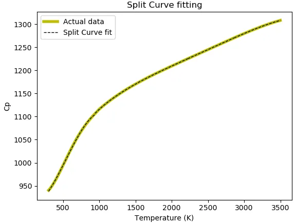
The yellow line represents the original plot.

The black dotted line represents the cubic fit.

Withe the help of splitwise fitting we have improved the cubic fit. We can verify it by comparing it with the earlier cubic plot.

Questions:

• What does popt & pcov mean?

popt represents the matrix which stores & extracts the coefficients for the fifitting functions according to the general equations defined.

popt array, Optimal values for the parameters so that the sum of the squared residuals of f(xdata, *popt) - ydata is minimized.

• What does np.array(temperature) do?

This comm& converts each value of temperature in the data le into an array using numpy module.

• What does the * in *popt mean?

'*' , '*popt' indicates & returns each coefficients stored in popt array. The * notation will exp& a list of values into the arguments of the function.

• What needs to be done in order to make the curve fit perfect?

Perfect fit means, the curve should fit the original curve without showing any errors in that particular degree of polynomial. This means that every data point in the original plot should be on the curve. Perfect fit can always be a best fit but best fit cannot be a perfect fit.

We can fit a curve perfectly only by using interpolation. It is not necessary that we get a single function representing complete trend.