Week 5 - Curve fitting

POPT and PCOV:

POPT-
It is an array of optimal values for any given set of parameters which minimizes the sum of squares of the residuals.
It basically defines an array of coefficients like function, temperature and Cp values.

PCOV-
It is known as the returned parameter covariance matrix.
It is a 2D array which consists an estimated covariance of the popt.
It is based on scaling sigma by a constant factor where sigma is scaled to match the sample variance of residuals after the fit.

np.array(temperature):

It basically brings out all the temperature values from the data file and places them in an array-grid format.
It's function is to set a grid of values which are non-negative integers.

* in *popt:

An asterix usually means a multiplication symbol, however here when it is inserted at the beginning of a variable, like an iterable or like a list/dictionary, it expands the contents of that variable and presents it.

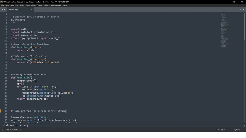
CODE TO FIT LINEAR AND CUBIC POLYNOMIAL FOR THE GIVEN Cp DATA:

• Import all relevant libraries.
• Define 2 seperate functions a and b for linear and cubic functions.
• Define another function to read the thromodynamic file.
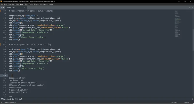
• Using popt, pcov and curve_fit commands write the main program for linear and cubic curve fitting.
• Using plt.plot command plot the given curves as shown in the code.
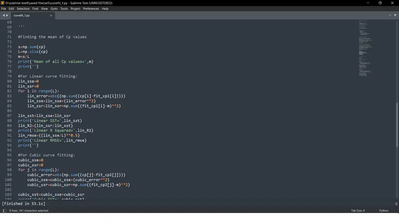
• For goodness of fit refer the comments on the code below.
• Assume sse/ssr=0 for both linear and cubic curves to be 0 and then using for loop write a code for the formula of the same.
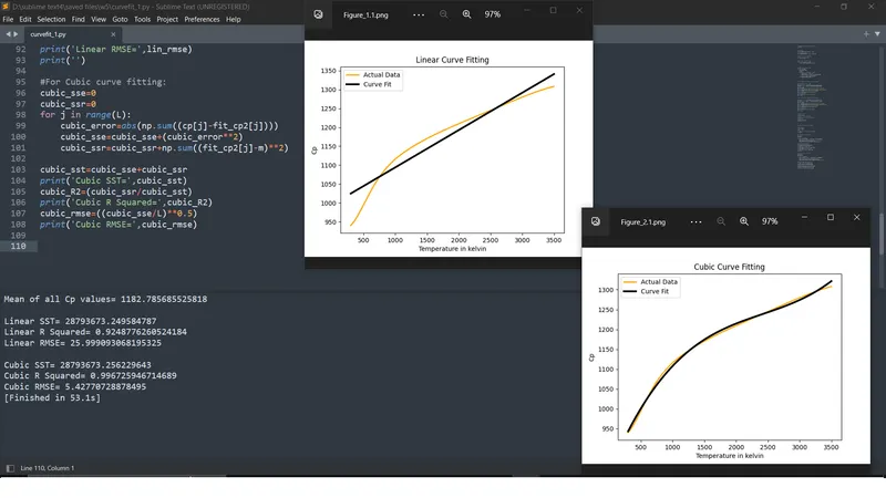
• Lastly, print all the values.

'''
To perform curve fitting on python
By Prithvi
'''

import math
import matplotlib.pyplot as plt
import numpy as np
from scipy.optimize import curve_fit 

#Linear Curve fit function:
def function_a(t,a,b):
	return a*t+b

#Cubic curve fit function:
def function_b(t,a,b,c,d):
	return a*(t**3)+b*(t**2)+c*t+d



#Reading thermo data file:
def read_file():
	temperature=[]
	cp=[]
	for line in open('data','r'):
		values=line.split(',')
		temperature.append(float(values[0]))
		cp.append(float(values[1]))
	return[temperature,cp]



# Main program for linear curve fitting:

temperature,cp=read_file()
popt,pcov=curve_fit(function_a,temperature,cp)
fit_cp1=function_a(np.array(temperature),*popt)
plt.figure(1)
plt.plot(temperature,cp,linewidth=2,color='orange')
plt.plot(temperature,fit_cp1,linewidth=3,color='black')
plt.legend(['Actual Data','Curve Fit'])
plt.xlabel('Temperature in kelvin')
plt.ylabel('Cp')
plt.title('Linear Curve Fitting')
plt.show()

# Main program for cubic curve fitting:

popt,pcov=curve_fit(function_b,temperature,cp)
fit_cp2=function_b(np.array(temperature),*popt)
plt.figure(2)
plt.plot(temperature,cp,linewidth=2,color='orange')
plt.plot(temperature,fit_cp2,linewidth=3,color='black')
plt.legend(['Actual Data','Curve Fit'])
plt.xlabel('Temperature in kelvin')
plt.ylabel('Cp')
plt.title('Cubic Curve Fitting')
plt.show()

'''
Goodness of fit:
 We know that,
SSE(sum of error squared)
SSR(sum of square of regression)
SST=SSE+SSR
R Squared=SSR/SST
RMSE=(SSE/L)*0.5

'''

#Finding the mean of Cp values

s=np.sum(cp)
L=np.size(cp)
m=s/L 
print('Mean of all Cp values=',m)
print('')

#For Linear curve fitting:
lin_sse=0
lin_ssr=0
for i in range(L):
	lin_error=abs((np.sum((cp[i]-fit_cp1[i]))))
	lin_sse=lin_sse+(lin_error**2)
	lin_ssr=lin_ssr+np.sum((fit_cp1[i]-m)**2)

lin_sst=lin_sse+lin_ssr
print('Linear SST=',lin_sst)
lin_R2=(lin_ssr/lin_sst)
print('Linear R Squared=',lin_R2)
lin_rmse=((lin_sse/L)**0.5)
print('Linear RMSE=',lin_rmse)
print('')

#For Cubic curve fitting:
cubic_sse=0
cubic_ssr=0
for j in range(L):
	cubic_error=abs(np.sum((cp[j]-fit_cp2[j])))
	cubic_sse=cubic_sse+(cubic_error**2)
	cubic_ssr=cubic_ssr+np.sum((fit_cp2[j]-m)**2)

cubic_sst=cubic_sse+cubic_ssr
print('Cubic SST=',cubic_sst)
cubic_R2=(cubic_ssr/cubic_sst)
print('Cubic R Squared=',cubic_R2)
cubic_rmse=((cubic_sse/L)**0.5)
print('Cubic RMSE=',cubic_rmse)

OUTPUT:

GRAPHS:

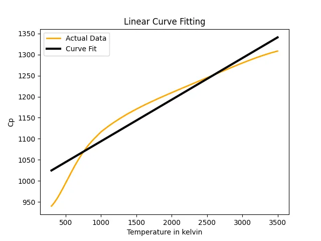
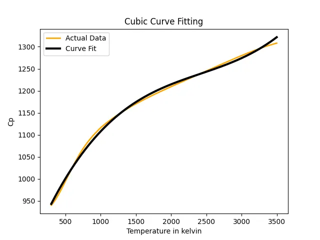
• The desired results were achieved. We were aiming to get a better fitted curve than what the linear equation produced hence we used a higher degree of polynomial namely, cubic and got the desired result of a better fitting curve from the actual data.
• To make the curve fit perfectly to the actual data several methods can be applied for example using a higher degree of polynomial than cubic however, sometimes it gets too complex and we don't get a better fitted curve and therefore we can use the splitwise method in which we basically split the cp and temperature values into equal parts and then plot them.
• As it is clearly visible in the graphs (Emperically clear) for linear and cubic fitting, the curve fits alot better for higher polynomial-cubic than the linear graph.

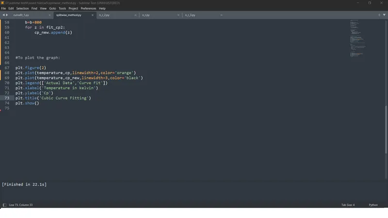
Please refer the images and code below for the splitwise method in detail for cubic curve fitting:

• For this method, copy the code until cubic curve.
• Assume a=0 and b=799---We basically divide all the data in the data file into 4 equal parts of 800 units each, so it's including 0 to 799 total is 800.
• Define a new cp array.
• Using a for loop to run it 4 times, we append the new cp value as shown below.
• Finally, plot the graph using new cp value.

'''
To perform curve fitting on python using splitwise method
By Prithvi
'''

import math
import matplotlib.pyplot as plt
import numpy as np
from scipy.optimize import curve_fit 

#Linear Curve fit function:
def function_a(t,a,b):
	return a*t+b

#Cubic curve fit function:
def function_b(t,a,b,c,d):
	return a*(t**3)+b*(t**2)+c*t+d



#Reading thermo data file:
def read_file():
	temperature=[]
	cp=[]
	for line in open('data','r'):
		values=line.split(',')
		temperature.append(float(values[0]))
		cp.append(float(values[1]))
	return[temperature,cp]



# Main program for linear curve fitting:

temperature,cp=read_file()
popt,pcov=curve_fit(function_a,temperature,cp)
fit_cp1=function_a(np.array(temperature),*popt)
plt.figure(1)
plt.plot(temperature,cp,linewidth=2,color='orange')
plt.plot(temperature,fit_cp1,linewidth=3,color='black')
plt.legend(['Actual Data','Curve Fit'])
plt.xlabel('Temperature in kelvin')
plt.ylabel('Cp')
plt.title('Linear Curve Fitting')
plt.show()

# Main program for cubic curve fitting using splitwise method:

a=0
b=799
cp_new=[]
for i in range(0,4):
	
	popt,pcov=curve_fit(function_b,temperature[a:b+1],cp[a:b+1])
	
	fit_cp2=function_b(np.array(temperature[a:b+1]),*popt)
	a=b+1
	b=b+800
	for z in fit_cp2:
		cp_new.append(z)
	



#To plot the graph:

plt.figure(2)
plt.plot(temperature,cp,linewidth=2,color='orange')
plt.plot(temperature,cp_new,linewidth=3,color='black')
plt.legend(['Actual Data','Curve Fit'])
plt.xlabel('Temperature in kelvin')
plt.ylabel('Cp')
plt.title('Cubic Curve Fitting')
plt.show()

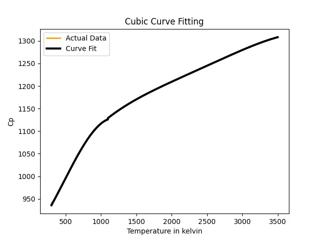
USING THE ABOVE COMMANDS BELOW IS THE OUTPUT ACHIEVED USING SPLITWISE METHOD FOR CUBIC CURVE FITTING:

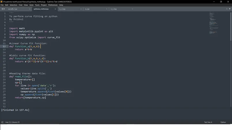
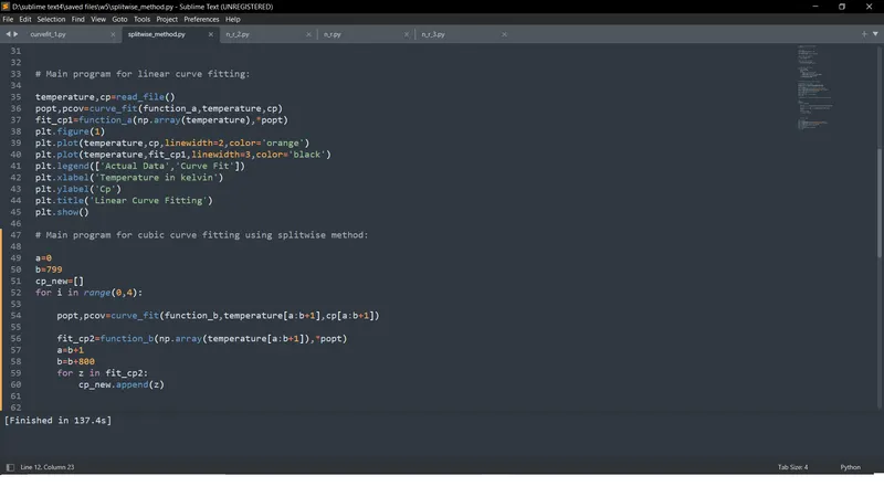
(USING SPLITWISE METHOD)

• As it is clearly shown in the graphs, splitwise method gives a much better fitted graph for cubic curve fitting.
• We can colclude that our cubic curve fits the actual data line almost perfectly.

NOTE: ALL FILES ARE ATTACHED IN .RAR FORMAT BELOW.