Week 5 - Curve fitting

Curve fitting- can be defined as the process of constructing a curve or mathematical function that has the best fit to a series of data points, subject to constraints.

In this project, the curve for Specific heat as a function of Temperature will be plotted and the plot will be compared with the actual plot.

The specific heats at different temperatures will be provided as inputs.

Initially, we will be writing a program for linear and cubic polynomial and check the results with the actual plot. Based on the results obtained, we are going to figure out the best possible ways to have a perfect fit.

popt: It gives an array with the optimal values for the parameters so that the sum of the squared residuals of data is minimized

pcov: It is a 2d array with the estimated covariance of the parameters in popt. It can be used to calculate the the standard deviation errors of popt.

np.array(temperature): This function stores the values of temperature in the form of array and passes it to the function numpy.

* in *popt: It stores the values of the constant parameters(a,b,c) in the array popt.

Program-

'''
 A program to determine fitness characteristics for the linear and cubic polynomial for the given Cp data
 By Sachin Barse
 '''

import math
import numpy as np
import matplotlib.pyplot as plt
from scipy.optimize import curve_fit


# Linear Curve fit function
def function_lcf(t, a, b):
    return a * t + b


# Cubic Curve fit function
def function_ccf(t, a, b, c, d):
    return a * pow(t, 3) + b * pow(t, 2) + c * t + d


# Reading thermodynamic data file
def read_file():
    temperature = []
    cp = []
    for line in open('data', 'r'):
        values = line.split(',')
        temperature.append(float(values[0]))
        cp.append(float(values[1]))

    return [temperature, cp]


# Main Program
temperature, cp = read_file()

popt, pcov = curve_fit(function_lcf, temperature, cp)
fit_cp_l = function_lcf(np.array(temperature), *popt)
plt.figure(1)
plt.plot(temperature, cp, 'b--')
plt.plot(temperature, fit_cp_l, color='red')
plt.legend(['Actual data', 'Curve fit'])
plt.xlabel('Temperature (K)')
plt.ylabel('Cp')
plt.title('Linear Curve fitting')
plt.show()

popt, pcov = curve_fit(function_ccf, temperature, cp)
fit_cp_c = function_ccf(np.array(temperature), *popt)
plt.figure(2)
plt.plot(temperature, cp, 'b--')
plt.plot(temperature, fit_cp_c, color='red')
plt.legend(['Actual data', 'Curve fit'])
plt.xlabel('Temperature (K)')
plt.ylabel('Cp')
plt.title('Cubic Curve fitting')
plt.show()


#Measuring the fitness characetristics of the curves

s = np.sum(cp)
l = np.size(cp)
m = s / l # Finding mean of Cp data
print('Mean of all cp :', m)
print('') #This will print an empty line (use to give line break)

# For Linear curve fit
linear_sse = 0
linear_ssr = 0
for i in range(l):
    linear_error = abs((np.sum((cp[i] - fit_cp_l[i]))))
    linear_sse = linear_sse + pow(linear_error, 2)
    linear_ssr = linear_ssr + np.sum(pow((fit_cp_l[i] - m), 2))

print('For Linear Curve Fit')
linear_sst = linear_sse + linear_ssr
print('linear_sst :', linear_sst)
linear_R2 = linear_ssr / linear_sst
print('linear_R2 :', linear_R2)
linear_rmse = pow((linear_sse / l), 0.5)
print('linear_RMSE :', linear_rmse)
print('') #This will print an empty line (use to give line break)

# For Cubic curve fit
cubic_sse = 0
cubic_ssr = 0
for j in range(l):
    cubic_error = abs(np.sum((cp[i] - fit_cp_c[i])))
    cubic_sse = cubic_sse + (pow(cubic_error, 2))
    cubic_ssr = cubic_ssr + np.sum(pow((fit_cp_c[i] - m), 2))

print('For Cubic Curve Fit')
cubic_sst = cubic_sse + cubic_ssr
print('cubic_sst :', cubic_sst)
cubic_R2 = cubic_ssr / cubic_sst
print('cubic_R2 :', cubic_R2)
cubic_rmse = pow((cubic_sse / l), 0.5)
print('cubic_RMSE :', cubic_rmse)

 

Steps-

First, we import some modules/libraries necessary for the code viz. math, numpy (as np), mathplotlib.pyplot (as plt) and from scipy.optimize we import curve_fit.

Then we define two function for linear curve fit and cubic curve fit. Later we read input file with the help of open command to open the file and ‘r’ to read the file. Then we extract temperature and cp by using line split (in this case it is separated by comma) to separate the data and return the values into their respective array (one for temperature and second for cp). We make use of append to append the data.

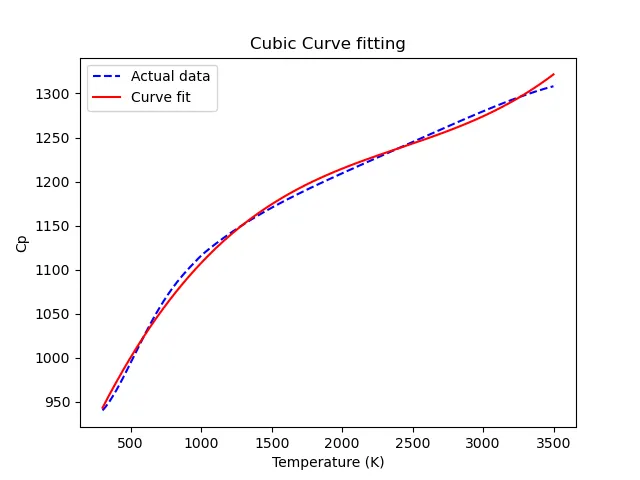
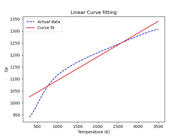
Then we come to our main code/program where we perform curve fit by using ‘curve_fit’ command which takes input as the required function (linear or cubic), temperature, and Cp. 'popt' and 'pcov' are used as output for storing parameters obtained by 'curve_fit'. Another variable named 'fit_cp' is used to stores the new values of Cp calculated by using temperature array. Plots of both raw dataset and predicted dataset are made and compared to find fitness characteristics for both the curves for both linear and cubic polynomial.

To measure the fitness characteristics for both the curves, various parameters such as Sum of Square Error (SSE), Sum of Square of the Regression (SSR), Sum of Square Total (SST), R-Square (R2), Root Mean Square Error (RMSE) are calculated. The plot which has highest R-Square (R2) or closest to 1 is considered to be a good fit.

Result -

Linear Curve Fit Plot

Cubic Curve Fit Plot