Week 5 - Curve fitting

AIM-

• Curve fitting

OBJECTIVE-

• Write code to fit a linear and cubic polynomial for the Cp data.
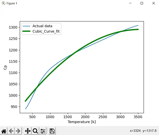
• Plot the linear and cubic fit curves along with the raw data points. Title and axes labels are a must, legends could be shown if necessary.
• Write a code to show split-wise method.
• Explain the parameters used to measure the fitness characteristics for both the curves.

THEORY-

Curve fitting is the process of constructing a curve, or mathematical functions, which possess the closest proximity to the real series of data. By curve fitting, we can mathematically construct the functional relationship between the observed dataset and parameter values, etc. It is highly effective in the mathematical modelling of some natural processes.

PROGRAM-

import math
import matplotlib.pyplot as plt
import numpy as np
from scipy.optimize import curve_fit

# curve fit function
# For linear equation
def func_0(t, a, b):
    return a*t + b

# for cubic equation
def func_1(t, a, b, c):
    return a*pow(t,2) + b*t + c

# for perfect closed fit equation
def func_2(t, a, b, c, d):
    return a*pow(t,3) + b*pow(t,2) + c*t + d

# Reading thermodynamic data file
def read_file():
    temperature = []
    cp = []
    for line in open('data','r'):
        values = line.split(',')
        temperature.append(float(values[0]))
        cp.append(float(values[1]))

    return[temperature, cp]

# Main program for Linear equation
temperature, cp = read_file()
popt, pcov = curve_fit(func_0, temperature, cp)
fit_cp = func_0(np.array(temperature), *popt)

plt.plot(temperature, cp)
plt.plot(temperature, fit_cp,color="red",linewidth=3.5)
plt.legend(['Actual data','Linear_Curve_fit'])
plt.xlabel('Temperature [k]')
plt.ylabel('Cp')
plt.show()

# Main program for Cubic equation
temperature, cp = read_file()
popt, pcov = curve_fit(func_1, temperature, cp)
fit_cp = func_1(np.array(temperature), *popt)

plt.plot(temperature, cp)
plt.plot(temperature, fit_cp,color="green",linewidth=3.5)
plt.legend(['Actual data','Cubic_Curve_fit'])
plt.xlabel('Temperature [k]')
plt.ylabel('Cp')
plt.show()

# Main program for Cubic equation
temperature, cp = read_file()
popt, pcov = curve_fit(func_2, temperature, cp)
fit_cp = func_2(np.array(temperature), *popt)

plt.plot(temperature, cp)
plt.plot(temperature, fit_cp,color="m",linewidth=3.5)
plt.legend(['Actual data','Perfect_Curve_fit'])
plt.xlabel('Temperature [k]')
plt.ylabel('Cp')
plt.show()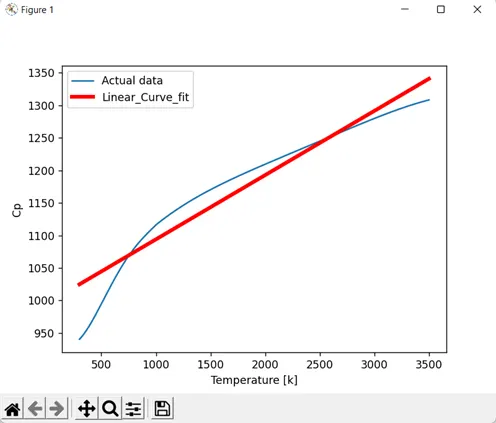

EXPLAINATION:

• We used required module like math, matplotlib, numpy, scipy module for python programming.
• As per given challenge, we defined two separate functions for linear and Cubic equation.
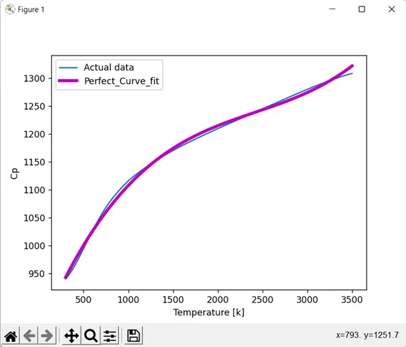
• Additionally, we trying to show perfect curve fit which is closed to given curve fit data file.
• To load given data file in python, first we save ‘data’ file in same location where we saved ‘Curve.py’ file means save file directory.
• To open, read and split given temperature and cp data, we used ‘for loop’ command.
• For curve fitting, we used ‘popt’ and ‘pcov’ as output for storing new temperature and cp data as input given function linear, cubic and perfect equation.
• For showing plotting, we used ”plot.show()” command. Here, we plot separate plot for linear, cubic and perfect curve which compare with Actual curve fit.

Question 1: What does popt and pcov means?

Answer: popt- It is a 1D array with optimal parameters generated by the equation given.

Pcov: It is a 2D array with estimated parameters from the popt generated.

Question 2: What does np.array (temperature) means?

Answer: The command ‘np.array(temperature)’, is used to convert the values of temperature parameter from given data file into an array. To execute this command, we used Numpy module.

Question 3: What does *popt means?

Answer: The *popt means, referring the values of popt in the program.

Question 4: What needs to be done in order to make the curve perfect?

Answer: To make the curve fit with the experimental value, we need to increase the order of polynomial equation.

Question 5: Show empirically as to how well your curve has been fit.

Answer:

Conclusion:

• Thus, the curve fit has been performed with polynomial and cubic polynomial equation fits with the experimental value given.
• We found that 4^th order of polynomial equation will gives closed fit.