Week 5 - Curve fitting

Aim:

Write a python code to perform Curve fit from a given data to compare it with experimental data

Solution:

1. What does popt and pcov mean?

popt: It's an 1D array with optimal parameters generated by equation given.

pcov: It’s a 2D array with an estimated parameters generated by popt.

2. What does np.array(temperature) do?

It will store the values of temperature in the form of array (temperature = [ ] ) from a given data file so that it can be used in the program later.

3. What does *popt means?

It refers the value of popt (coefficients of equation) in the program.

4. What needs to be done in order to make the curve perfect?

One can use the higher order of polynomial or vice versa.

Program:

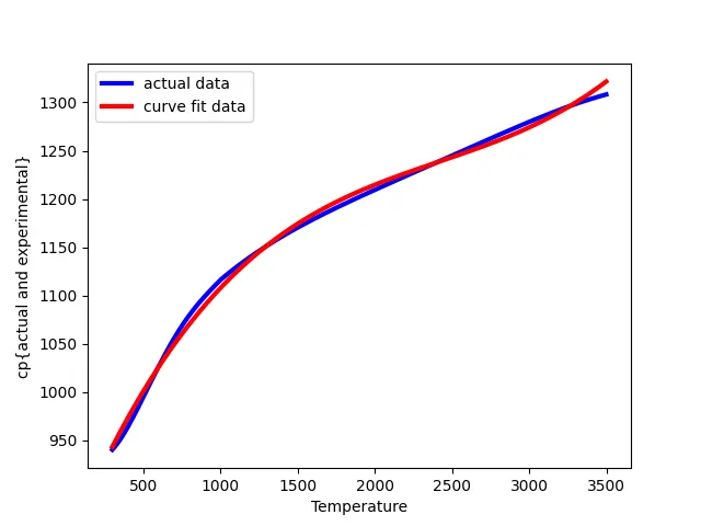
1. for cubic polynomial equation

#Curve Fit in Python
#Anvar Choksi 

import math 
import matplotlib.pyplot as plt 
import numpy as np 
from scipy.optimize import curve_fit 

#Curve fit function 
def func(t,a,b,c,d):
	return a*pow(t,3) + b*pow(t,2) + c*t + d 

def read_file():
	temperature = []
	cp = []

	for line in open('data','r'):
		values = line.split(',')
		temperature.append(float(values[0]))
		cp.append(float(values[1]))

	return [temperature,cp]

#Main program 
temperature,cp = read_file()
popt,pcov = curve_fit(func,temperature,cp)
fit_cp = func(np.array(temperature), *popt)

plt.plot(temperature,cp,color='blue',linewidth= 3)
plt.plot(temperature,fit_cp,color='red',linewidth= 3)
plt.legend(["actual data", "curve fit data"])
plt.xlabel("Temperature")
plt.ylabel("cp{actual and experimental}")
plt.show()

2. For Linear Equation:

#Curve Fit in Python
#Anvar Choksi 

import math 
import matplotlib.pyplot as plt 
import numpy as np 
from scipy.optimize import curve_fit 

#Curve fit function 
def func(t,a,b):
	return a*t + b

def read_file():
	temperature = []
	cp = []

	for line in open('data','r'):
		values = line.split(',')
		temperature.append(float(values[0]))
		cp.append(float(values[1]))

	return [temperature,cp]

#Main program 
temperature,cp = read_file()
popt,pcov = curve_fit(func,temperature,cp)
fit_cp = func(np.array(temperature), *popt)

plt.plot(temperature,cp,color='blue',linewidth= 3)
plt.plot(temperature,fit_cp,color='red',linewidth= 3)
plt.legend(["actual data", "curve fit data"])
plt.xlabel("Temperature")
plt.ylabel("cp{actual and experimental}")
plt.show()

Conclusion:

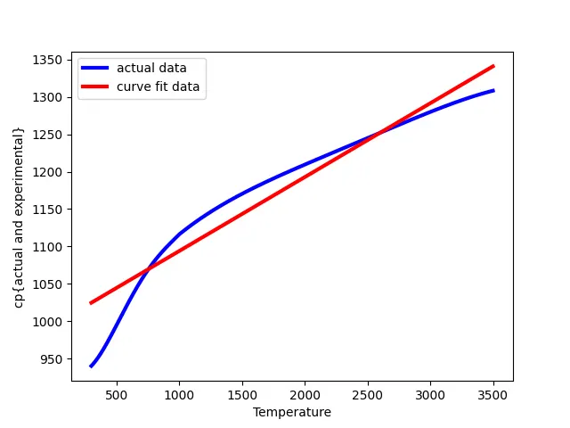
It can be seen from the plots that the cubic polynomial equation curve fits with the data given.