Week 5 - Curve fitting

Aim: To write the code to fit the linear and cubic polynomial for the given cp data.

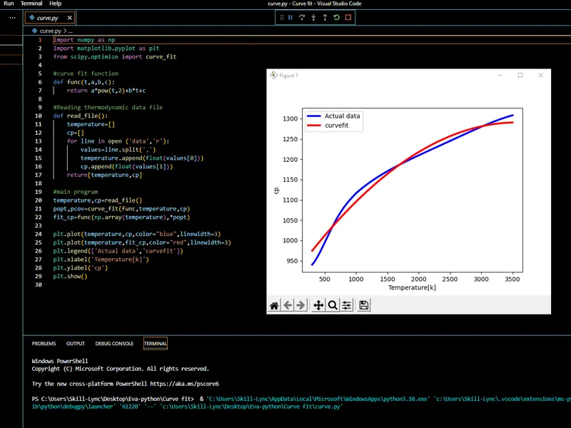
Program:(2nd order)

import numpy as np
import matplotlib.pyplot as plt
from scipy.optimize import curve_fit

#curve fit function
def func(t,a,b,c):
    return a*pow(t,2)+b*t+c

#Reading thermodynamic data file
def read_file():
    temperature=[]
    cp=[]
    for line in open ('data','r'):
        values=line.split(',')
        temperature.append(float(values[0]))
        cp.append(float(values[1]))
    return[temperature,cp]

#main program
temperature,cp=read_file()
popt,pcov=curve_fit(func,temperature,cp)
fit_cp=func(np.array(temperature),*popt)

plt.plot(temperature,cp,color="blue",linewidth=3)
plt.plot(temperature,fit_cp,color="red",linewidth=3)
plt.legend(['Actual data','curvefit'])
plt.xlabel('Temperature[k]')
plt.ylabel('cp')
plt.show()

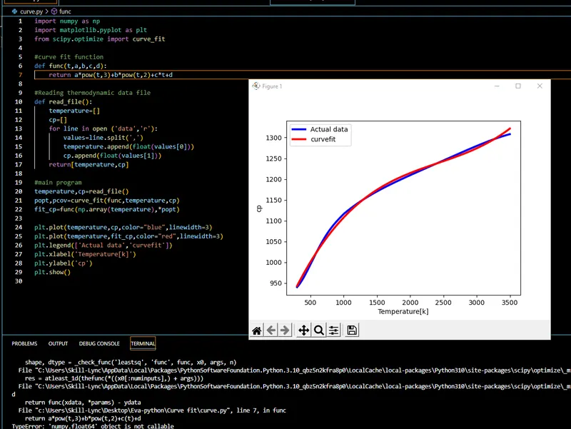
Program:(3rd order)

import numpy as np
import matplotlib.pyplot as plt
from scipy.optimize import curve_fit

#curve fit function
def func(t,a,b,c,d):
    return a*pow(t,3)+b*pow(t,2)+c*t+d

#Reading thermodynamic data file
def read_file():
    temperature=[]
    cp=[]
    for line in open ('data','r'):
        values=line.split(',')
        temperature.append(float(values[0]))
        cp.append(float(values[1]))
    return[temperature,cp]

#main program
temperature,cp=read_file()
popt,pcov=curve_fit(func,temperature,cp)
fit_cp=func(np.array(temperature),*popt)

plt.plot(temperature,cp,color="blue",linewidth=3)
plt.plot(temperature,fit_cp,color="red",linewidth=3)
plt.legend(['Actual data','curvefit'])
plt.xlabel('Temperature[k]')
plt.ylabel('cp')
plt.show()

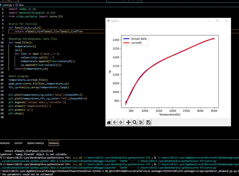
Program:(4th order)

import numpy as np
import matplotlib.pyplot as plt
from scipy.optimize import curve_fit

#curve fit function
def func(t,a,b,c,d,e):
    return a*pow(t,4)+b*pow(t,3)+c*pow(t,2)+d*t+e

#Reading thermodynamic data file
def read_file():
    temperature=[]
    cp=[]
    for line in open ('data','r'):
        values=line.split(',')
        temperature.append(float(values[0]))
        cp.append(float(values[1]))
    return[temperature,cp]

#main program
temperature,cp=read_file()
popt,pcov=curve_fit(func,temperature,cp)
fit_cp=func(np.array(temperature),*popt)

plt.plot(temperature,cp,color="blue",linewidth=3)
plt.plot(temperature,fit_cp,color="red",linewidth=3)
plt.legend(['Actual data','curvefit'])
plt.xlabel('Temperature[k]')
plt.ylabel('cp')
plt.show()

Explanation:

Initially the given dtat file is downloaded and stored in the same folder where the program codefor the curve fit is saved.

Next the function statement for the given is obtained.

Defining of the function with time t and the unknown coefficients are done.

Calling of the function using the read_file is done.

While calling a function through read_file it calls the temperature and the cp value stoed in the data file.

That is done through initialization of the empty array for temperature[] and cp[].

Here for command is given to open a data file and to read 'r' is given.

for line in open('data','r'):

Next 3 different commands are given for the same program,

values=line.split(',')

in the above command 2 data values is split with help of comma

temperature.append(float(values[0]))

in the above command the index is zero

cp.append(float(values[1]))

in the above command indexed value is 1.

Casting these as float values is done since these are stored as strings and in order to read a string we need float.

And once after adding float append is used to add the values resulted in an empty array.

Finally return the values in an array.

Now under the main program,

popt is the output function which stores the unknown coefficient a,b,c.

Answers:

1.Popt is an array that stores the coefficient of an equation with respect to the polynomial degree.

pcov is a 2D array that consists of covariance of popt. Covariance gives the relation between 2 values.

2. An array is the collection of items stored at contiguous memory locations. The idea is to store multiple items of the same type together. In python,the array command is stored in a module called numpy.

3. popt is an array which consists of all the coefficient of equation generated based on the degree of the polynomial. popt is the command which gives the same coefficient of the equation but it will multiply with e and give the output.

5. To make a curve fit perfectly the estimates should be taken into account. The perfect fit is the one which matches the original curve irrespective of any scaling and centering errors in that particular degree of polynomial. The R^2 value must be equal to 1 and the sum of squares due to error(SSE)=0.

Screenshots:

Result:

The code is scripted for the various polynomial order for the given data and the curve fitting plot is also obtained for all 2nd, 3rd and 4th polynomial order.