Week 3 - Solving second order ODEs
Aim: To write a program that simulate the pendulum motion in the form 2nd order ODE given.
Given parameters:
L=1 metre,
m=1 kg,
b=0.05.
g=9.81 m/s2.
Simulation to be carried out for the motion between 0-20 sec, for angular displacement=0,angular velocity=3 rad/sec at time t=0.
Program:
clear all
close all
clc

%step1:input
%damping coefficient
b=0.02;
%gravity of earth
g=9.81;
%length of rope/string
l=1;
%mass of ball
m=0.1;

%step2:initial condition for displacement and angular velocity
theta_0 = [0;3]

%step3:time interval points
t_span = linspace(0,20,500);

%step4:ODE results
%call ode_fun function
%ode45 gives result in rad & rad/s
[t,result] = ode45(@(t,theta)ode_fun(t,theta,b,g,l,m),t_span,theta_0);

%step5:plotting
figure(1)
plot(t,result(:,1))
hold on
plot(t,result(:,2))
title('for simple pendulum')
xlabel('time in sec')
ylabel('angular velocity(rad/s)/displacement(rad)')
legend('displacement','angular velocity')

%step6:animation of pendulum
amplitude = result(:,1);%store amplitude values in separate matrix for loop
p=1;
for i=1;length(amplitude)
    angle=amplitude(i);
    firgure(2)
    title('simple pendulum')

    %fix point of pendulum
    x0=0;
    y0=0;
    %another end of pendulum/coordinate of mass ball
    x1 = l*sin(angle);
    y1 =-l*cos(angle);
    %plot
    plot([-1.1 1.1],[0 0],'linewidth',2);%celling line
    hold on
    plot([x0 x1],[y0 y1],'color','g','linewidth',2)%string
    plot(x1,y1,'0','markers',20,'markerfacecolor',[1 1 0])%mass ball
    hold off %removing previous position
    grid on
    axis([-1.5 1.5 -1.5 0.5])
    pause(0.001)
    M(P) = getframe(gcf);
    P = P+1;
end
Explanation:
The transient behaviour of the system is described by the help of Ordinary Partial Differential equation.
Step1:
Damping coeeficient vale is given b=0.02
Weight that pull down the force due to gravity and it is given as g=9.81m/s^2
Length of the string that hold the ball is 1meter
Mass of the ball is 1kg and it is given as m=0.1
Step2:
Initial condition for displacement and angular velocity is declared in this step.
theta in terms of displacement and velocity is assigned with values 0,3
Step3:
Time interval points is assigned in the time array with the command linspace and the values 0,20,500 is given for the same.
Step4:
ODE function is called in, in order to obtain the result in terms of displacement and angular velocity.
t,result is the time variation with ode45 which is a inbuilt software and ode_fun is the matlab code for the function and finally the intial parameter with dependent and independent variables.
Step5:
Final plot for the same is obtained with both displacement and velocity and by changing the damping value changes in the graph can be observed.
Step6:
Animation is created for the pendulum with the plot data in the M(P) = getframe(gcf)
Axis is defined as [-1.5 1.5 -1.5 1.5]
Step7:
The animation is saved on the desktop and updated to the you tube in the videofile.
Link is obtained from the same in uncompressed avi format.
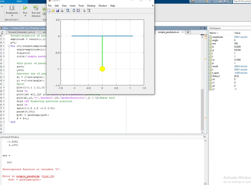
Screenshot of the error faced:
Steps taken:
Defined a value for the variable P, in the initial parameters where inputs were assisgned .
Final program:
clear all
close all
clc

%step1:input
%damping coefficient
b=0.02;
%gravity of earth
g=9.81;
%length of rope/string
l=1;
%mass of ball
m=0.1;
P=1

%step2:initial condition for displacement and angular velocity
theta_0 = [0;3]

%step3:time interval points
t_span = linspace(0,20,500);

%step4:ODE results
%call ode_fun function
%ode45 gives result in rad & rad/s
[t,result] = ode45(@(t,theta)ode_fun(t,theta,b,g,l,m),t_span,theta_0);

%step5:plotting
figure(1)
plot(t,result(:,1))
hold on
plot(t,result(:,2))
title('for simple pendulum')
xlabel('time in sec')
ylabel('angular velocity(rad/s)/displacement(rad)')
legend('displacement','angular velocity')

%step6:animation of pendulum
amplitude = result(:,1);%store amplitude values in separate matrix for loop
p=1;
figure(2)
for i=1:length(amplitude)
    angle=amplitude(i);
    title('simple pendulum')

    %fix point of pendulum
    x0=0;
    y0=0;
    %another end of pendulum/coordinate of mass ball
    x1 = l*sin(angle);
    y1 =-l*cos(angle);
    %plot
    plot([-1.1 1.1],[0 0],'linewidth',2);%celling line
    hold on
    plot([x0 x1],[y0 y1],'color','g','linewidth',2)%string
    plot(x1,y1,'o','markers',20,'markerfacecolor',[1 1 0])%mass ball
    hold off %removing previous position
    grid on
    axis([-1.5 1.5 -1.5 0.5])
    pause(0.001)
    M(P) = getframe(gcf);
    P = P+1;
end

%step7:making movie
movie(M)
videofile=VideoWriter('simple_pendulum.avi','uncompressed avi');
open(videofile)
writeVideo(videofile,M)
close(videofile)
Result:
The program for the second order ODE is solved and the you tube link with the animation for the same is attached below.