Week 2 Air standard Cycle

Aim:To write code that can solve an otto cycle and make plots for it.

1. Code should create a PV diagram

2. Should output the thermal efficiency of the engine.

Program code:

"""
Engine kinematics
"""
import math
import matplotlib
#geometric parameters
bore=0.10
stroke=0.1
con_rod=0.15
cr=12
a = stroke/2
R = con_rod/a

#volume parameters
v_s = math.pi*(1/4)*pow(bore,2)*stroke
v_c = v_s/(cr-1)

theta = math.radians(0)
term1 = 0.5*(cr-1)
term2 = R+1-math.cos(theta)
term3 = pow(R,2)-pow(math.sin(theta),2)
term3 = pow(term3,0.5)

V = (1+term1*(term2-term3))*v_c
print(v_c)
print(V)

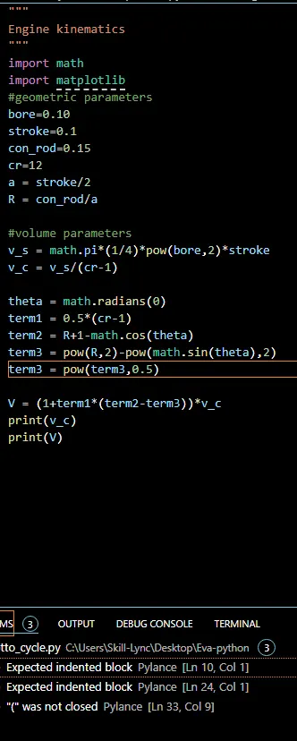
Error screenshot:

Steps taken to overcome the errors:

1. Spacing of the code check is made to recitify the errors.

final program:

import math
import matplotlib.pyplot as plt

def engine_kinematics(bore,stroke,con_rod,cr,start_crank,end_crank):
	
	a=stroke/2
	R=con_rod/a
	n=100
	

	sc=math.radians(start_crank)
	ec=math.radians(end_crank)
	dtheta=(ec-sc)/(n-1)
	v=[]
	for i in range(0,n):
		theta=sc+i*dtheta
		term1=(0.5*(cr-1))
		term2=R+1-math.cos(theta)
		term3=pow(R,2)-pow(math.sin(theta),2)
		term3=pow(term3,0.5)

		v.append((1+term1*(term2-term3))*v_c)
	return v

bore=0.1
stroke=0.12
con_rod=0.15
cr=12

#INPUTS
p1=101325
t1=500
gamma=1.4
t3=2300
th_eff=(1-1/pow(cr,gamma-1))*100
print(th_eff)
v_s=math.pi/4*pow(bore,2)*stroke
v_c=v_s/(cr-1)
v1=v_s+v_c

#STATE POINTS 2
v2=v_c
p2=p1*pow(v1,gamma)/pow(v2,gamma)

#P2V2/T2=P1V1/T1  | rhs=P1V1/T1   |	P2V2/T2=rhs   | T2=P2V2/rhs

rhs=p1*v1/t1
t2=p2*v2/rhs

v_compression=engine_kinematics(bore,stroke,con_rod,cr,180,0)
constant=p1*pow(v1,gamma)
p_compression=[]

for v in v_compression:
	p_compression.append(constant/pow(v,gamma))

#STATE POINTS 3
v3=v2
rhs=p2*v2/t2
p3=rhs*t3/v3

v_expansion=engine_kinematics(bore,stroke,con_rod,cr,180,0)
constant=p3*pow(v3,gamma)
p_expansion=[]

for v in v_expansion:
	p_expansion.append(constant/pow(v,gamma))

#STATE POINTS 4
v4=v1
p4=p3*pow(v3,gamma)/pow(v4,gamma)
t4=p4*v4/rhs

plt.plot([v2,v3],[p2,p3])
plt.plot(v_compression, p_compression)
plt.plot(v_expansion,p_expansion)
plt.plot([v4,v1],[p4,p1])
plt.show()
plt.savefig('pvdiagram.png')

Explanation:

For otto cycle the following process are considered

1-2 Isentropic compression

2-3 Constant volume heat addition

3-4 Isentropic expansion

4-1 Constant volume heat rejection

Engine geometric parameters,

Bore,stroke,connecting rod length,cr are defined with values.

Outputs for the same is declared in terms of v1,t1,p1,v2,t2,p2,v3,t3,p3,cr

Formula to determine how the volume inside the IC engine change:

V/Vc = 1+(0.5)(rc-1)[R+1-cos theta-(R²-sin² theta)]

Swept volume and clearance volume is also defined for the air standard cycle.

The formula for the IC engine also split into multiple terms to ease the solvation.

State variables at point 1 2 3 4 are also declared

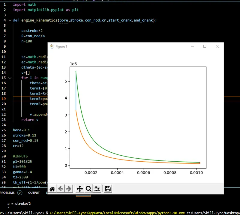
Plotting for the same is done.

Screenshot of the output:

Result:

Plot for the otto cycle is obtained.