Week 4.1 - Genetic Algorithm
Aim : To write a code in MATLAB to optimise the stalagmite function and find the global maxima of the function.
Program code:
clear all
close all
clc

%define searcg space
x = linspace(0,0.6,150);
y = linspace(0,0.6,150);
n = 50;

%creating a 2D mesh
[xx yy] = meshgrid(x,y);

%evaluating a stalagmite function
for i=1:length(xx)
    for j=1:length(yy)
        input_vector(1) = xx(i,j);
        input_vector(2) = yy(i,j);
        f(i,j) = stalagmite(input_vector);
    end
end

%study1: statistical behaviour
tic
for i=1:n
    [inputs,fopt(i)] = ga(@stalagmite,2);
    xopt(i) = inputs(1);
    yopt(i) = inputs(2);
end
study1_time = toc

figure(1)
subplot(2,1,1)
hold on
surfc(xx,yy,-f)
shading interp
xlabel('x-axis')
ylabel('y-axis')
title('statistical behaviour with unbound inputs')
plot3(xopt,yopt,-fopt,'marker','o','markersize',5,'markerfacecolor','r')
subplot(2,1,2)
plot(-fopt)
xlabel('no of iterations')
ylabel('function maximum')

%study2: statistical behaviour with upper and lower bounds
tic
for i=1:n
    [inputs,fopt(i)] = ga(@stalagmite,2,[],[],[],[],[0:0],[1:1]);
    xopt(i) = inputs(1);
    yopt(i) = inputs(2);
end
study2_time = toc

figure(2)
subplot(2,1,1)
hold on
surfc(xx,yy,-f)
shading interp
xlabel('x-axis')
ylabel('y-axis')
title('statistical behaviour with upper and lower bounds')
plot3(xopt,yopt,-fopt,'marker','o','markersize',5,'markerfacecolor','r')
subplot(2,1,2)
plot(-fopt)
xlabel('no of iterations')
ylabel('function maximum')

%study3: statistical behaviour with increasing iterations of GA
options = optimoptions('ga');
options = optimoptions(options,'population size',300);
xopt(i) =inputs(1);
yopt(i) =inputs(2);

study3_time = toc
figure(3)
subplot(2,1,1)
hold on
surfc(xx,yy,-f)
shading interp
xlabel('x-axis')
ylabel('y-axis')
title('statistical behaviour with increasing iterations')
plot3(xopt,yopt,-fopt,'marker','o','markersize',5,'markerfacecolor','r')
subplot(2,1,2)
plot(-fopt)
xlabel('no of iterations')
ylabel('function maximum')
Explanation:
Genetic algorithm generates a population o0f points at each iteration. The best point in the population approaches an optimal solution as it selects the next population by computation which uses random number generates.
In order to define stalagmite function,need to write a different script defining the stalagmite function.
The whole term of function is split into multiplpe small terms and written interms of equation as follows.
t1=(sin((5.1*pi*x)+0.5))^6;
t2=(sin((5.1*pi*y)+0.5))^6;
t3=exp(-4*log(2)*((x-0.0667)^2)/0.64);
t4=exp(-4*log(2)*((y-0.0667)^2)/0.64);
Creating a 2D mesh is carried out with help of the command meshgrid
for loop to evaluate a stalagmite function is stated with the input vector in xx and yy function.
Study 1: statistical behaviour
tic is the input command given and calling of the function interms of the ga is done.
Plot of the output is labelled in the x and y axis. Also sub plots for the same is included in the same program code.
Study 2: Statistical behaviour with upper and lower bounds
Arrays are declared for the ga function defined to obtain the output in the same manner.
markersize markerfacecolor all defined while plotting the output graphs.
Iterations for the program is also labelled along with x axis and the function maximum is labelled in the y axis.
Study 3: Statistical behaviour with increasing iterations of GA
optimooptions are defined in this stage.
xopt for the input and yopt for input 2 is defined.
toc is another output command with respect to time end program.
Plotting is carried out for the same.
Error code and screenshot: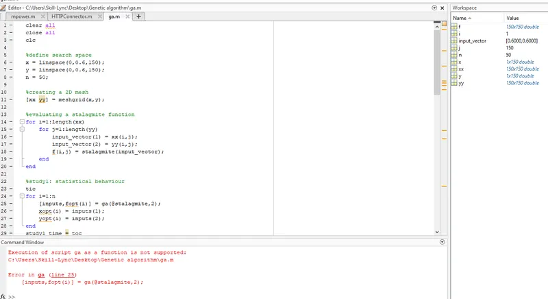
Steps taken to overcome the error:
Carried out the installation of Optimization toolbox and global optimization toolbox.
Final program:(Function code)
%define stalagmite function

function[f] = stalagmite(input_vector)
x = input_vector(1);
y = input_vector(2);

t1 =(sin((5.1*pi*x)+0.5))^6;
t2 =(sin((5.1*pi*y)+0.5))^6;
t3 =exp(-4*log(2)*((x-0.0667)^2)/0.64);
t4 =exp(-4*log(2)*((y-0.0667)^2)/0.64);

f =-(t1*t2*t3*t4);
end
Final program:(Main code)
clear all
close all
clc

%define search space
x = linspace(0,0.6,150);
y = linspace(0,0.6,150);
n = 15;

%creating a 2D mesh
[xx, yy] = meshgrid(x,y);

%evaluating a stalagmite function
for i=1:length(xx)
    for j=1:length(yy)
        input_vector(1) = xx(i,j);
        input_vector(2) = yy(i,j);
        f(i,j) = stalagmite(input_vector);
    end
end
% surfc(x,y,f)
%study1: statistical behaviour
tic
for i=1:n
    [inputs,fopt(i)] = ga(@stalagmite,2);
    xopt(i) = inputs(1);
    yopt(i) = inputs(2);
end
fopt=-fopt;
study1_time = toc

figure(1)
subplot(2,1,1)
hold on
surfc(x,y,-f)
shading interp
plot3(xopt,yopt,fopt,'marker','o','markersize',5,'markerfacecolor','r')
title('unbound inputs')
% figure(2)
subplot(2,1,2)
plot(fopt)
xlabel('Iterations')
ylabel('function maximum')

%study2: statistical behaviour with upper and lower bounds
tic
for i=1:n
    [inputs2,fopt2(i)] = ga(@stalagmite,2,[],[],[],[],[0:0],[0.6:0.6]);
    xopt2(i) = inputs2(1);
    yopt2(i) = inputs2(2);
end
fopt2=-fopt2;
study2_time = toc

figure(2)
subplot(2,1,1)
hold on
surfc(x,y,-f)
shading interp
plot3(xopt2,yopt2,fopt2,'marker','o','markersize',5,'markerfacecolor','r')
title('Bounded inputs')
%figure(2)
subplot(2,1,2)
plot(fopt2)
xlabel('Iterations')
ylabel('function maximum')

%study3: statistical behaviour with increasing iterations of GA
options = optimoptions('ga');
options = optimoptions(options,'populationsize',500);
tic
for i=1:n
    [inputs3,fopt3(i)] = ga(@stalagmite,2,[],[],[],[],[0:0],[0.6:0.6],[],options);
    xopt3(i) = inputs3(1);
    yopt3(i) = inputs3(2);
end

study3_time = toc
figure(3)
subplot(2,1,1)
hold on
surfc(x,y,-f)
shading interp
plot3(xopt3,yopt3,-fopt3,'marker','o','markersize',5,'markerfacecolor','r')
title('Bounded inputs with optioptims function')
subplot(2,1,2)
plot(-fopt3)
xlabel('Iterations')
ylabel('function minimum')

study3_time = toc
rng('default')
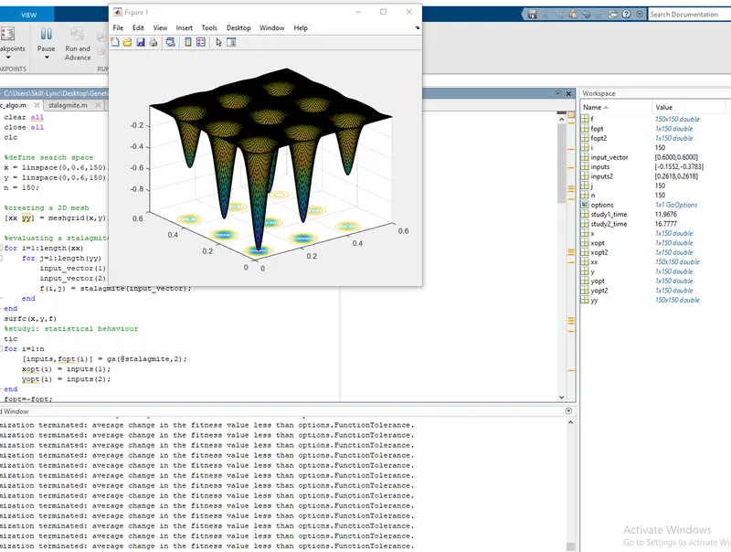
Screenshot 1:
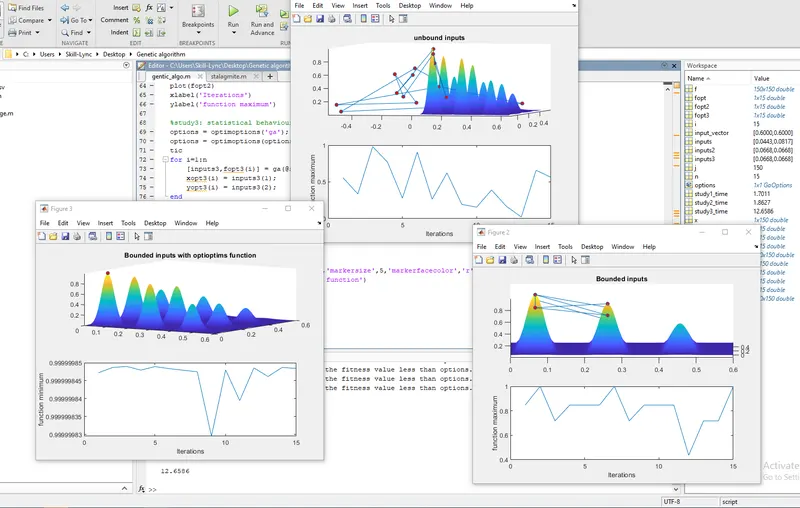
Screenshot 2:
Result:
The concept of genetic algorithm regarding stalagmite function and ways to optimise it is carried out.
The code to optimise the stalagmite function and find the global maxima of the function is done using MATLAB.
The resultant graph are attached for the same.