Week 5 - Curve fitting

Aim:

To program about Curve fitting using python

INTRODUCTION:

Curve fit are useful to discribe how your data changes,It is the process of consturctively curve or mathematical function,which posses the closet proximity to the real series of data, we can mathematically construct the functional relatioship between the observed dataset and parameters values.

CODE EXPLANATION:

• Importing the useful liberaries math, matplotlib, numpy and scipy module to be installed.
• define the function for liner polynomial (a*t+b), and then read the file
• download the data file
• what does the arry of temperature do
• now creating two empty arrays for temperature and cp values to be stored.
• now opeing the data file to reading mode
• using line.split(,) this will divide the line into two part, the comma will allow the temperature and cp data in seprate arrays.
• the temperature wil index as 0 and cp as 1
• we make the float case the value in the dataare in the form of string
• now we return the value of temperature and cp back to the function
• What does the popt, pcov means
• The popt command is used to argument contains the best fit parameters for the varaibles a and b.
• The pcov variable contain covariance matrix, which indicates uncertainalbe and correalation between parameters
• what does *in popt do
• now using the function again to fit the curve taking the temp values from array and the values of a,b from (*popt) this *in and *popt use the value a,b store in popt amd use them while making plot
• this will use for cubic polynomial also

CODE:

import math
import numpy as np
import matplotlib.pyplot as plt
from scipy.optimize import curve_fit

# function of curve fitting
def func(t,a,b):
return a*t + b

# Reading thermodynamics file data

def read_file():
temperature = []
cp = []
for line in open('data','r'):
values = line.split(' , ')
temperature.append(float(values[0]))
cp.append(float(values[1]))
return (temperature,cp)

# main program
temperature,cp = read_file()
popt, pcov = curve_fit(func, temperature, cp)
fit_cp = func(np.array(temperature), *popt)
print(popt)
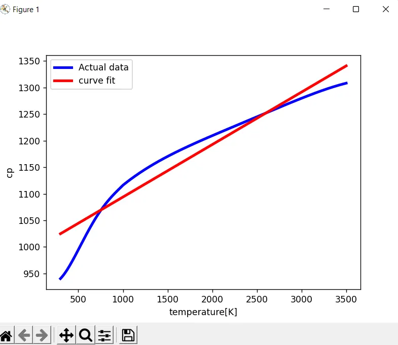
plt.plot(temperature,cp,color= 'blue',linewidth = 3)
plt.plot(temperature,fit_cp,color= 'red',linewidth = 3)
plt.legend(['Actual data', 'curve fit'])
plt.xlabel('temperature[K]')plt.ylabel('cp')
plt.show()

CUBIC polynomial :

import math
import numpy as np
import matplotlib.pyplot as plt
from scipy.optimize import curve_fit

# function of curve fitting
def func(t, a, b, c, d):
return a*pow(t,3) + b*pow(t,2) + c*t +d

# Reading thermodynamics file data

def read_file():
temperature = []
cp = []
for line in open('data','r'):
values = line.split(' , ')
temperature.append(float(values[0]))
cp.append(float(values[1]))
return (temperature,cp)

# main program
temperature,cp = read_file()
popt, pcov = curve_fit(func, temperature, cp)
fit_cp = func(np.array(temperature), *popt)
print(popt)
plt.plot(temperature,cp,color= 'blue',linewidth = 3)
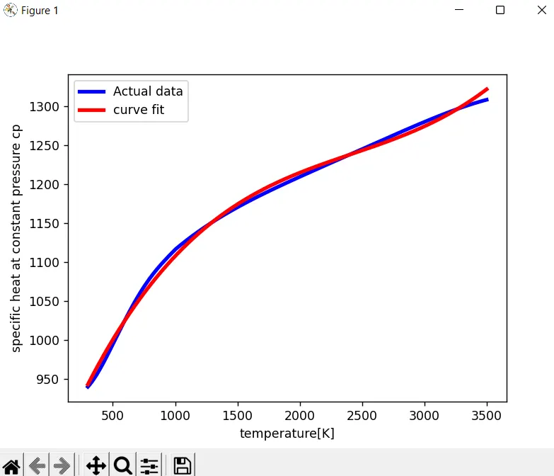
plt.plot(temperature,fit_cp,color= 'red',linewidth = 3)
plt.legend(['Actual data', 'curve fit'])
plt.xlabel('temperature[K]')
plt.ylabel('specific heat at constant pressure cp')
plt.show()

OUTPUT:

plot as actual data vs linear fit

OUTPUT:

plot as actual data vs curve fit

RESULT :

• step to make the curve fit perfect
• the mathematical curve has some variant from the original curve it means it has some error in the value of varaible (a,b,c,d) in the equation.