Project 2 - Rankine cycle Simulator
AIM:
create a Rankine cycle simulator using MATLAB
OBJECTIVE:
- calculate each state point of the Rankine cycle(any type of your choice) based on user inputs
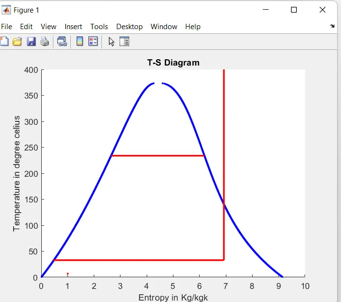
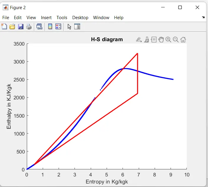
- plot corresponding T-s and h-s plot for the given set of inputs
- calculate Efficiency
Note: The standard XSteam library is used to get the steam table data for water is given, which is used to calculate the point in between the state variable.
THEORY:
- The rankine cycle converts thermal energy to mechanical energy
- On-road vechicles, which convert around one-third of the fuel energy into useful mechanical energy for propulsion, are moving energy conversion system that generate consuderable waste heat
- It is found from prior research that the rankine cycle has great potential in automobile waste harvesting application which can, in turn,be connected to the combustion engine which will result in better-wasted heat consumption and increasing the performance of the vechile and helping the environment.
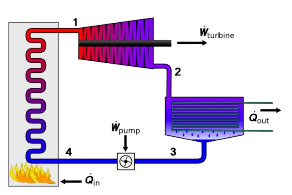
- The ideal rankine cycle consist of the following four process
- 1-2:Isentropic compression in a pump
- 2-3 Constant pressure heat addition in a boiler
- 3-4 Isentropic expansion in a turbine
- 4-1 constant pressure heat rejection in a codenser
Procedure:
1. First, all the required variables and parameters were foi=und out to calcuate
2. Then,using the"XSTeam" library function, all the parameter were sorted out.
3. Then, the usual calculation and plotting of the graphs were done as per the theory of thermodynamics.
MATLAB PROGRAM:
clear all
close all
clc
% point process description
fprintf('\n1-2 Isentropic expansion in the turbine\n')
fprintf('2-3 Constant Pressure heat rejection by the condenser expansion\n')
fprintf('3-4 Isentropic compression in pump \n')
fprintf('4-1 Constant Pressure heat addition by the boiler \n')
%Enter Inputs
P1 = input('Enter the pressure at the turbine inlet (in bar):');
T1 = input('Enter the temperature at the turbine inlet (in degree celius):');
P2 = input('Enter the pressure at the condensor (in bar):');
%calculate each state point XSteam values
%state point 1
H1 = XSteam('h_pt',P1,T1);
S1 = XSteam('s_pt',P1,T1);
Sf1= XSteam('sL_p',P1);
Sg1 = XSteam('sV_p',P1);
Hf1 = XSteam('hL_p',P1);
Hg1 = XSteam('hV_p',P1);
Ts1 = XSteam('Tsat_p',P1);
%state point2
S2 = S1;
Sf2 = XSteam('sL_p',P2);
Sg2 = XSteam('sV_p',P2);
x =(S2-Sf2)/(Sg2-Sf2);
Hf2 = XSteam('hL_p',P2);
Hg2 = XSteam('hV_p',P2);
H2 = Hf2 + x*(Hg2-Hf2);
T2 = XSteam('T_hs',H2,S2);
%state point3
T3 = T2;
P3 = P2;
S3 = Sf2;
H3 = Hf2;
%state point 4
P4 = P1;
S4 = S3;
H4 = XSteam('h_ps',P4,S4);
T4 = XSteam('T_ps',P4,S4);
%temp space for plotting saturation curves
t = linspace(0,374,500);
%plot T-S diagram
figure(1)
hold on
%plot saturation curve
for i = 1:length(t)
plot(XSteam('sL_T',t(i)),t(i),'.','Color','b');
plot(XSteam('sV_T',t(i)),t(i),'.','Color','b');
end
%plot cycle
plot([S1 S2],[T1 T2],'LineWidth',2,'color','r');
if x>1
T3 = Ts2;
plot([S2 Sg2 S3 S4],[T2 ts2 T3 T4],'LineWidth',2,'color','r');
T2 = Ts2;
else
plot([S2 S3 S4],[T2 T3 T4],'LineWidth',2,'color','r');
end
l = linspace(T1,T2,1000);
for i = 1:length(1)
plot(XSteam('s_pT',P1,l(i)),'.','color','r')
end
plot([Sf1 Sg1],[Ts1 Ts1],'linewidth',2,'color','r')
xlabel('Entropy in Kg/kgk')
ylabel('Temperature in degree celius')
title('T-S Diagram')
%plot H-S diagram
figure(2)
hold on
for i= 1:length(t)
plot(XSteam('sL_T',t(i)),XSteam('hL_T',t(i)),'.','Color','b')
plot(XSteam('sV_T',t(i)),XSteam('hV_T',t(i)),'.','Color','b')
end
plot([S1 S2 S3 S4 S1],[H1 H2 H3 H4 H1],'LineWidth',2,'Color','r');
xlabel('Entropy in Kg/kgk')
ylabel('Enthalpy in KJ/Kgk')
title('H-S diagram')
%calculate other output values
%turbine works
wt = H1-H2;
%pump works
wp = H4-H3;
%net work
w_net = wt - wp;
%heat addition
Qin = H1-H4;
%heat rejection
Qout = H2-H3;
%efficiency
N_Therm = (w_net/Qin)*100;
%specific steam consumption
Steam_rate = 3600/(w_net);
%Back work ratio
BWR = wp/wt;
%point all state point values to show
fprintf('\n______Result______\n')
fprintf('At state point 1:\n')
fprintf('P1 is : %.2f bar\n',P1)
fprintf('T1 is : %.2f deg celius\n',T1)
fprintf('H1 is : %.2f KJ/Kg\n',H1)
fprintf('S1 is : %.2f KJ/Kg-K\n',S1)
fprintf('At state point 2:\n')
fprintf('P2 is : %.2f bar\n',P2)
fprintf('T2 is : %.2f deg celius\n',T2)
fprintf('H2 is : %.2f KJ/Kg\n',H2)
fprintf('S2 is : %.2f KJ/Kg-K\n',S2)
fprintf('At state point 3:\n')
fprintf('P3 is : %.2f bar\n',P3)
fprintf('T3 is : %.2f deg celius\n',T3)
fprintf('H3 is : %.2f KJ/Kg\n',H3)
fprintf('S3 is : %.2f KJ/Kg-K\n',S3)
fprintf('At state point 4:\n')
fprintf('P4 is : %.2f bar\n',P4)
fprintf('T4 is : %.2f deg celius\n',T4)
fprintf('H4 is : %.2f KJ/Kg\n',H4)
fprintf('S4 is : %.2f KJ/Kg-K\n',S4)
fprintf('\nwt is :%2f KJ/Kg\n',wt)
fprintf('wp is :%2f KJ/Kg\n',wp)
fprintf('w_net is :%2f KJ/Kg\n',w_net)
fprintf('Thermal_Efficiency is : %.2f percent\n',N_Therm)
fprintf('Steam_rate. is : %.2f Kg/Kwh\n',Steam_rate)
fprintf('Back Work Ratio is : %.3f \n',BWR)
Command window:
1-2 Isentropic expansion in the turbine
2-3 Constant Pressure heat rejection by the condenser expansion
3-4 Isentropic compression in pump
4-1 Constant Pressure heat addition by the boiler
Enter the pressure at the turbine inlet (in bar):30
Enter the temperature at the turbine inlet (in degree celius):400
Enter the pressure at the condensor (in bar):0.05
______Result______
At state point 1:
P1 is : 30.00 bar
T1 is : 400.00 deg celius
H1 is : 3231.57 KJ/Kg
S1 is : 6.92 KJ/Kg-K
At state point 2:
P2 is : 0.05 bar
T2 is : 32.88 deg celius
H2 is : 2110.71 KJ/Kg
S2 is : 6.92 KJ/Kg-K
At state point 3:
P3 is : 0.05 bar
T3 is : 32.88 deg celius
H3 is : 137.77 KJ/Kg
S3 is : 0.48 KJ/Kg-K
At state point 4:
P4 is : 30.00 bar
T4 is : 32.95 deg celius
H4 is : 140.76 KJ/Kg
S4 is : 0.48 KJ/Kg-K
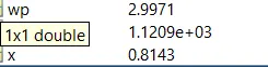
wt is :1120.862815 KJ/Kg
wp is :2.997107 KJ/Kg
w_net is :1117.865709 KJ/Kg
Thermal_Efficiency is : 36.17 percent
Steam_rate. is : 3.22 Kg/Kwh
Back Work Ratio is : 0.003
Result graph:
T-S Diagram
H-S Diagram
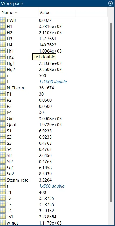
Workspace:
Errors:
A minor error was taken, were didnt save my xsteam table, that's the problem
Conclusion:
- The rankine cycle is basic cycle for steam turbine system in thermodynamics
- The required output values are obtained
- net work output = 1117.87kj/Kg
- Back work ratio = 0.0027
- Thus, the rankine cycle is successfully simulated in Matlab