Week 5 - Curve fitting

Aim: To write a program in python in curve fitting using linear and cubic polynomial from the provided data.

Theory: Curve fitting is used to find the best fit curve for a series of data points. It helps in capturing the trend in the data by assigning a single function across the entire range. Once the model is created, we can check the goodness of the curve using four parameters.

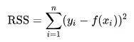
1. Sum of Squares Error (SSE) - sum of the squares of the deviations predicted from the actual values from the data.
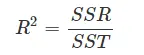
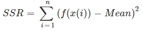
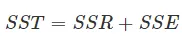
2. R-square : It is the measure of how close the data are fitted to the regression line.
3. Adjusted R-square: It is the modified version of R-square corresponding to the number of predictions made.
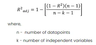
4. Root mean square error: It measures the average magnitude of the errors.

Program (Linear polynomial):

import numpy as np
import numpy
import matplotlib.pyplot as plt
from scipy.optimize import curve_fit


#Polynomial function

def fun_lin(t,a,b):
    return a*t + b


#Function to read the file
def read_file():
    temp=[]
    cp=[]
    for line in open('data','r'):
        data_split=line.split(',')
        temp.append(float(data_split[0]))
        cp.append(float(data_split[1]))
    return [temp,cp]


#Main program
temp,cp=read_file()
popt,pcov=curve_fit(fun_lin,temp,cp)
fitted_cp=fun_lin(np.array(temp),*popt)

#Plotting
plt.plot(temp,cp,linewidth=4,color="red")
plt.plot(temp,fitted_cp,linewidth=4,color="green")
plt.legend(['Actual Curve','Fitted Curve'])
plt.xlabel('Temperature in K')
plt.ylabel('Speific Heat in kJ/kgK')
plt.title('Linear Curve Fitting')
plt.show()


#Calculating error and goodness
length=len(temp)
for i in range(length):
    error=cp-fitted_cp
    sse=pow(error,2)
    rmse_val=sse/6
    rmse=pow(rmse_val,0.5)
    mean=numpy.asarray(cp[i])/numpy.asarray(i)
    ssr=pow(numpy.asarray(cp[i])-numpy.asarray(mean),2)
    sst=ssr+sse
    r_square=ssr/sst
    print(r_square)

Explanation:

• open - read the data from the file provided.
• data_split - data storage and splitted as temperature and cp accordingly.
• append - to put the values in the array.
• fun_lin - function provided.
• popt - it contains the coefficients for the linear function (a,b), which are the best fit parameters.
• pcov - it contains the true variance and covariance of the parameters, from which we can find the standard deviation.

Program (for cubic polynomial):

import numpy as np
import numpy
import matplotlib.pyplot as plt
from scipy.optimize import curve_fit


#Polynomial function

def fun_lin(t,a,b,c,d):
    return a*pow(t,3) + b*pow(t,2)+c*t+d


#Function to read the file
def read_file():
    temp=[]
    cp=[]
    for line in open('data','r'):
        data_split=line.split(',')
        temp.append(float(data_split[0]))
        cp.append(float(data_split[1]))
    return [temp,cp]


#Main program
temp,cp=read_file()
popt,pcov=curve_fit(fun_lin,temp,cp)
fitted_cp=fun_lin(np.array(temp),*popt)

#Plotting
plt.plot(temp,cp,linewidth=4,color="red")
plt.plot(temp,fitted_cp,linewidth=4,color="green")
plt.legend(['Actual Curve','Fitted Curve'])
plt.xlabel('Temperature in K')
plt.ylabel('Speific Heat in kJ/kgK')
plt.title('Cubic Curve Fitting')
plt.show()


#Calculating error and goodness
length=len(temp)
for i in range(length):
    error=cp-fitted_cp
    sse=pow(error,2)
    rmse_val=sse/6
    rmse=pow(rmse_val,0.5)
    mean=numpy.asarray(cp[i])/numpy.asarray(i)
    ssr=pow(numpy.asarray(cp[i])-numpy.asarray(mean),2)
    sst=ssr+sse
    r_square=ssr/sst
    print(r_square)

Result:

(1) Linear fit curve

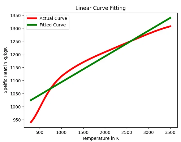
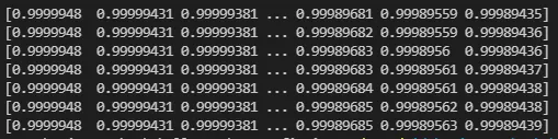
The obtained R-square values are in the range of 0.994 - 0.999, which results in a good fit.

(2) Cubic fit curve:

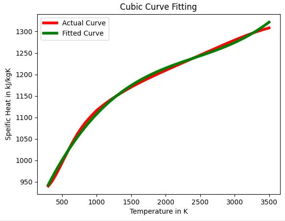
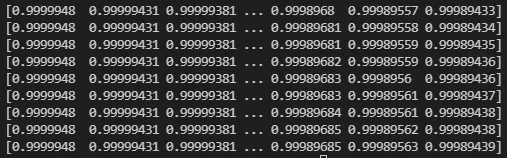
Here, the obtained R-square value is in the range of 0.999, which reslts in a perfect fit.

Conclusion:

On increasing the order of the polynomial, the curve becomes more fitter.