Week 5 - Curve fitting
Objective: - To write a python program to perform linear and polynomial curve fitting for a given data, empirically showcase the goodness of fit and make the curve fit perfect.
Problem Statement: -
1. What does popt and pcov mean?
2. What does np.array(temperature) do?
3. What does the * in *popt mean?
4. Write code to fit a linear and cubic polynomial for the Cp data. Explain if your results are good or bad.
5. What needs to be done in order to make the curve fit perfect?
6. Show empirically as to how well your curve has been fit.
Theory: - Curve fitting is a process where real sets of data are represented by a best possible curve or mathematical function. Curve fitting allows us to visualize data, predict values of a function where no data is availabe and to form relationship between two or more variables.
There are various type of curve fittings:
1. Linear curve fitting
2. Polynomial curve fitting
A straight line equation is fitted to a set of data in the first type while a polynomial function is fitted to a set of data in the latter type.
Following are the four parameters that help us to determine the goodness of the fits:
1. Sum of squared errors(SSE)
2. R-square
3. Adjusted R-square
4. Root Mean Squared Error(RMSE)
Governing Equation: -
Sum of squared errors(SSE) = `SSE=∑_(i=1)^n(Y(i)-f(x(i) ))^2`
Sum of squared of the regression(SSR) = `SSR=∑_(i=1)^n(f(x(i) )- Mean)^2`
Total sum of the squares(SST) = SSE+SSR
R-square = `R^2=SSR//SST`
Solution Procedure:-
# CODE1: TO FIT A LINEAR AND CUBIC POLYNOMIAL FOR THE Cp DATA.
- "Numpy", "math" and "matplotlib" library are imported to perform array, mathematical operations and to plot graphs respectively.
- From "scipy.optimize" library "curve_fit" function is imported to perform curve fitting in python.
- A user-defined function 'read_file' is created to read the thermodynamic data file containing temperature and specific heat values.
- Two empty variables 'temperature' and 'Cp' are created and using "for loop" and "line" as a counter variable each line containing a set od temperature and Cp values are opened line by line.
- A variable named 'values' is created and using the "split" function data in each line are splitted into two columns at the ',' argument.
- Using the "append" function, the empty arrays temperature, Cp are appended with values[0] and values[1] respectively and using return function they are returned to the function.
- The function 'read_file' is called to get the temperature and specific heat values.
- A user-defined function 'linear' is created with t,a,b as the input arguments to perform curve fitting using linear polynomial.
- The curve fitting is performed using the 'curve_fit' function. Same is done for the cubic polynomial by creating a user-defined function 'cubic' is created with t,a,b,c,d as the input arguments
- Finally, the plots between actual data and curve fit data are plotted for two of the cases.
# TO WRITE A PYTHON PROGRAM TO PERFORM CURVE FITTING USING LINEAR AND CUBIC POLYNOMIAL.
# SUBMITTED BY IRFAN SUNNY BARUAH ON 30/03/2022.
# CODE1: TO FIT A LINEAR AND CUBIC POLYNOMIAL FOR THE Cp DATA.
#=======================================================================================================
import math
import numpy as np
import matplotlib.pyplot as plt
from scipy.optimize import curve_fit
#--------------------------------------------------------------------------------------------------------
# Defining a function to read the thermodynamic data file containing temperature and specific heat values.
def read_file():
	temperature = []
	Cp =[]
	for line in open('data','r'):
		values = line.split(',')
		temperature.append(float(values[0]))
		Cp.append(float(values[1]))
	return [temperature, Cp]
#--------------------------------------------------------------------------------------------------------
# Calling the function read_file to get the temperature and specific heat values.
temperature, Cp = read_file()
#--------------------------------------------------------------------------------------------------------
# Performing curve fitting using linear polynomial.
# Defining the linear curve fitting function.
def linear(t,a,b):
	return a*t+b
# Performing curve fitting using the 'curve_fit' function and calling the 'linear' function
popt_linear, pcov_linear = curve_fit(linear, temperature, Cp)
linear_fit_cp = linear(np.array(temperature), *popt_linear)
#---------------------------------------------------------------------------------------------------------
# PLOTTING OF THE ACTUAL DATA AND THE LINEAR CURVE FIT DATA.
# Creating an empty figure.
plt.figure(1)
# Creating the plot between temperature and Cp.
plt.plot(temperature,Cp, color = 'red', linewidth = 2)
# Creating the plot between temperature and linear_fit_cp.
plt.plot(temperature, linear_fit_cp,color = 'black', linewidth = 2)
# Giving the title to the plot.
plt.title('Curve fitting using linear polynomial', fontname ="Times New Roman", fontsize = 10, fontweight = 'bold')
# Adding legends to the plot
plt.legend(['Actual data', 'Curve fit'])
# Adding grid lines to the plot
plt.grid()
# Adding x and y label to the polot
plt.xlabel('Temperature[K]')
plt.ylabel('Specific Heat[KJ/Kg-K]')
# Saving the figure
plt.savefig('Curve fitting using linear polynomial')
#------------------------------------------------------------------------------------------------------------
# Performing curve fitting using cubic polynomial.
# Defining the cubic curve fitting function
def cubic(t,a,b,c,d):
	return a*pow(t,3)+b*pow(t,2)+c*t+d
# Performing curve fitting using the 'curve_fit' function and calling the 'cubic' function.
popt_cubic, pcov_cubic = curve_fit(cubic, temperature, Cp)
cubic_fit_cp = cubic(np.array(temperature), *popt_cubic)
#-------------------------------------------------------------------------------------------------------------
# PLOTTING OF THE ACTUAL DATA AND THE CUBIC CURVE FIT DATA.
# Creating an empty figure.
plt.figure(2)
# Creating the plot between temperature and Cp.
plt.plot(temperature,Cp, color = 'red', linewidth = 2)
# Creating the plot between temperature and cubic_fit_cp.
plt.plot(temperature, cubic_fit_cp, color = 'black', linewidth = 2)
# Giving the title to the plot.
plt.title('Curve fitting using cubic polynomial', fontname ="Times New Roman", fontsize = 10, fontweight = 'bold')
# Adding legends to the plot.
plt.legend(['Actual data', 'Curve fit'])
# Adding grid lines to the plot.
plt.grid()
# Adding x and y label to the plot.
plt.xlabel('Temperature[K]')
plt.ylabel('Specific Heat[KJ/Kg-K]')
# Saving the figure.
plt.savefig('Curve fitting using cubic polynomial')
# CODE2: TO CALCULATE THE R-SQUARE VALUE TO SHOW HOW WELL THE CURVES HAS BEEN FIT.
- "Numpy", "math" and "matplotlib" library are imported to perform array, mathematical operations and to plot graphs respectively.
- From "scipy.optimize" library "curve_fit" function is imported to perform curve fitting in python.
- A user-defined function 'read_file' is created to read the thermodynamic data file containing temperature and specific heat values.
- Two empty variables 'temperature' and 'Cp' are created and using "for loop" and "line" as a counter variable each line containing a set od temperature and Cp values are opened line by line.
- A variable named 'values' is created and using the "split" function data in each line are splitted into two columns at the ',' argument.
- Using the "append" function, the empty arrays temperature, Cp are appended with values[0] and values[1] respectively and using return function they are returned to the function.
- The function 'read_file' is called to get the temperature and specific heat values.
- A user-defined function 'linear' is created with t,a,b as the input arguments to perform curve fitting using linear polynomial.
- The curve fitting is performed using the 'curve_fit' function. Same is done for the cubic polynomial by creating a user-defined function 'cubic' is created with t,a,b,c,d as the input arguments.
- Finally, the values of R-square for linear and cubic polynomial are calculated according to the above equations.
# TO WRITE A PROGRAM TO SHOW EMPIRICALLY THE GOODNESS OF FIT OF LINEAR AND CUBIC POLYNOMIAL.
# SUBMITTED BY IRFAN SUNNY BARUAH ON 30/03/2022.
# CODE2: TO CALCULATE THE R-SQUARE VALUE TO SHOW HOW WELL THE CURVES HAS BEEN FIT.
#==========================================================================================================
import math
import numpy as np
import matplotlib.pyplot as plt
from scipy.optimize import curve_fit
#---------------------------------------------------------------------------------------------------------
# Defining a function to read the thermodynamic data file containing temperature and specific heat values.
def read_file():
	temperature = []
	Cp =[]
	for line in open('data','r'):
		values = line.split(',')
		temperature.append(float(values[0]))
		Cp.append(float(values[1]))
	return [temperature, Cp]
# Calling the function read_file to get the temperature and specific heat values
temperature, Cp = read_file()
#----------------------------------------------------------------------------------------------------------
# Performing curve fitting using linear polynomial
# Defining the linear curve fitting function
def linear(t,a,b):
	return a*t+b
# Performing curve fitting using the 'curve_fit' function and calling the 'linear' function.
popt_linear, pcov_linear = curve_fit(linear, temperature, Cp)
linear_fit_cp = linear(np.array(temperature), *popt_linear)
#----------------------------------------------------------------------------------------------------------
# R-square value for linear polynomial.
# Calculating the sum of squared errors.
SSE = np.sum(pow(np.array(np.array(Cp)- np.array(linear_fit_cp)),2))
# Calculating the sum of squared of regression.
SSR = np.sum(pow(np.array(np.array(linear_fit_cp)- np.mean(Cp)),2))
# Calculating the total sum of the squares.
SST = SSR + SSE
# Calculating the R-sqaure value.
R_square_linear = SSR/SST
# Printing the R-square value.
print('The value of R-square for linear polynomial =', R_square_linear )
#-----------------------------------------------------------------------------------------------------------
# Performing curve fitting using cubic polynomial.
# Defining the cubic curve fitting function
def cubic(t,a,b,c,d):
	return a*pow(t,3)+b*pow(t,2)+c*t+d
# Performing curve fitting using the 'curve_fit' function and calling the 'cubic' function.
popt_cubic, pcov_cubic = curve_fit(cubic, temperature, Cp)
cubic_fit_cp = cubic(np.array(temperature), *popt_cubic)
#----------------------------------------------------------------------------------------------------------
# R-square value for cubic polynomial.
# Calculating the sum of squared errors.
SSE = np.sum(pow(np.array(np.array(Cp)- np.array(cubic_fit_cp)),2))
# Calculating the sum of squared of regression.
SSR = np.sum(pow(np.array(np.array(cubic_fit_cp)- np.mean(Cp)),2))
# Calculating the total sum of the squares.
SST = SSR + SSE
# Calculating the R-sqaure value.
R_square_cubic = SSR/SST
# Printing the R-square value.
print('The value of R-square for cubic polynomial =', R_square_cubic )
# CODE3: PERFORMING SPLITWISE METHOD TO MAKE THE CURVE FIT PERFECT.
- "Numpy", "math" and "matplotlib" library are imported to perform array, mathematical operations and to plot graphs respectively.
- From "scipy.optimize" library "curve_fit" function is imported to perform curve fitting in python.
- A user-defined function 'read_file' is created to read the thermodynamic data file containing temperature and specific heat values.
- Two empty variables 'temperature' and 'Cp' are created and using "for loop" and "line" as a counter variable each line containing a set od temperature and Cp values are opened line by line.
- A variable named 'values' is created and using the "split" function data in each line are splitted into two columns at the ',' argument.
- Using the "append" function, the empty arrays temperature, Cp are appended with values[0] and values[1] respectively and using return function they are returned to the function.
- The function 'read_file' is called to get the temperature and specific heat values.
- The temperature and Cp arrays are broken down into four arrays of equal lengths.
- A user-defined function 'cubic' is created with t,a,b,c,d as the input arguments to perform curve fitting of the four ranges.
- The curve fitting is performed using the 'curve_fit' function and the 'cubic_fit_cp' of all the ranges are concatenated.
- Finally, the plots between actual data and curve fit data found by splitwise method are plotted.
# TO WRITE A PYTHON PROGRAM TO PERFORM SPLITWISE METHOD OF CURVE FITTING.
# SUBMITTED BY IRFAN SUNNY BARUAH ON 30/03/2022.
# CODE3: PERFORMING SPLITWISE METHOD TO MAKE THE CURVE FIT PERFECT.
#===========================================================================================================
import math
import numpy as np
import matplotlib.pyplot as plt
from scipy.optimize import curve_fit
#-----------------------------------------------------------------------------------------------------------
# Defining a function to read the thermodynamic data file containing temperature and specific heat values.
def read_file():
	temperature = []
	Cp =[]
	for line in open('data','r'):
		values = line.split(',')
		temperature.append(float(values[0]))
		Cp.append(float(values[1]))
	return [temperature, Cp]
# Calling the function read_file to get the temperature and specific heat values
temperature, Cp = read_file()
#-----------------------------------------------------------------------------------------------------------
# Breaking down the temperature and Cp arrays into four arrays of equal lengths.
# Temperature and Cp values in range of 1 to 800.
temp1 = temperature[0:800]
Cp1 = Cp[0:800]
# Temperature and Cp values in range of 801 to 1600.
temp2 = temperature[800:1600]
Cp2 = Cp[800:1600]
# Temperature and Cp values in range of 1601 to 2400.
temp3 = temperature[1600:2400]
Cp3 = Cp[1600:2400]
# Temperature and Cp values in range of 2401 to 3200.
temp4 = temperature[2400:3200]
Cp4 = Cp[2400:3200]
#------------------------------------------------------------------------------------------------------------
# Performing curve fitting using cubic polynomial for the above ranges.
# Defining the cubic curve fitting function.
def cubic(t,a,b,c,d):
	return a*pow(t,3)+b*pow(t,2)+c*t+d
# Curve fitting for Range[1-800]
popt_cubic1, pcov_cubic1 = curve_fit(cubic, temp1, Cp1)
cubic_fit_cp1 = cubic(np.array(temp1), *popt_cubic1)
# Curve fitting for Range[801-1600]
popt_cubic2, pcov_cubic2 = curve_fit(cubic, temp2, Cp2)
cubic_fit_cp2 = cubic(np.array(temp2), *popt_cubic2)
# Curve fitting for Range[1601-2400]
popt_cubic3, pcov_cubic3 = curve_fit(cubic, temp3, Cp3)
cubic_fit_cp3 = cubic(np.array(temp3), *popt_cubic3)
# Curve fitting for Range[2401-3200]
popt_cubic4, pcov_cubic4 = curve_fit(cubic, temp4, Cp4)
cubic_fit_cp4 = cubic(np.array(temp4), *popt_cubic4)
# Concatenating the 'cubic_fit_cp' of all the ranges.
splitwise_cp = np.concatenate((cubic_fit_cp1,cubic_fit_cp2,cubic_fit_cp3,cubic_fit_cp4))
#---------------------------------------------------------------------------------------------------------------
# Creating an empty figure.
plt.figure()
# Creating a plot between temperature and Cp.
plt.plot(temperature,Cp, ls ='--', color = 'red', linewidth = 2)
# Creating a plot between temperature and splitwise_cp.
plt.plot(temperature,splitwise_cp, color = 'black', linewidth = 2)
# Giving title to the plot.
plt.title('Splitwise Method of Curve fitting', fontname ="Times New Roman", fontsize = 10, fontweight = 'bold')
# Adding legned to the plot.
plt.legend(['Actual data', 'Curve fit'])
# Adding x and y labels to the plot.
plt.xlabel('Temperature[K]')
plt.ylabel('Specific Heat[KJ/Kg-K]')
# Adding grid lines to the plot.
plt.grid()
# Saving the plot
plt.savefig('Splitwise Method of Curve fitting')
#================================================================================================================
Result and Discussion: -
1. The inbuilt 'curve_fit' function returns two output arguments 'popt' and 'pcov'. The first one is an array that contains best fit parameters(coefficients) of a polynomial so that the sum of the squared residuals for a given data is minimized. The latter is a 2D array which gives the estimated covariance of popt. The diagonals provide the variance of the parameter estimate. To compute one standard deviation errors of a given set of data, pcov can be used.
Fig1 - popt and pcov for linear polynomial
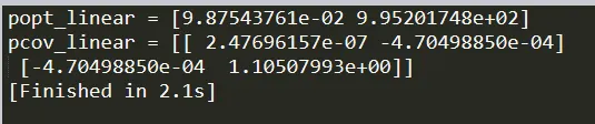
Fig2 - popt and pcov for cubic polynomial

2 The command 'np.array(temperature)' aids in accessing each and every element in the temperature array for elementwise operation.
3. The * in *popt simply helps to access the best fit parameters in the popt array. Basically, the * is referring to all the elements in the array.
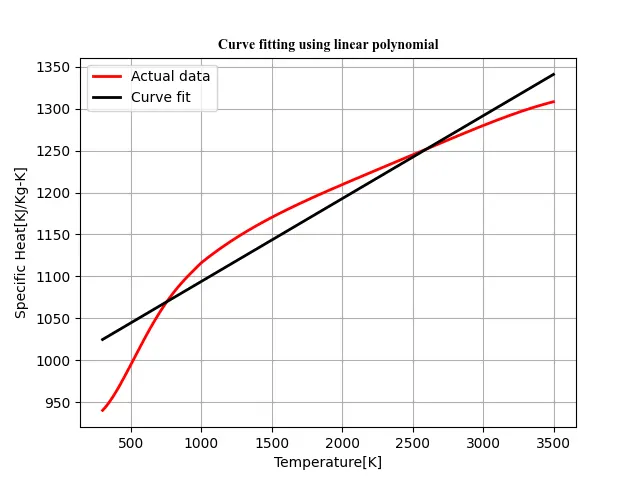
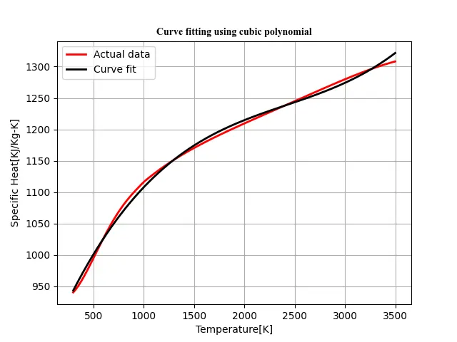
4. The curve fitting using linear and cubic polynomial has been carried out successfully. From the below graphs, the cubic polynomial results appear to be good.
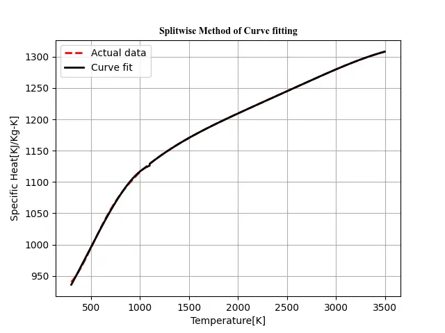
5. The splitwise method is performed and following is the plot of the code.
6. In order to show empirically whether the linear or cubic polynomial is a better fit or not, R - square value is calculated and it can be seen from the below figure that the value of R -square for cubic polynomial is close to 1. Therefore, the cubic polynomial represents the data better as compared to linear resulting in less errors in prediction of future values.
Fig3 - R-square value for linear and cubic polynomial.

.