Week 2 Air standard Cycle

Objective: - To write a python program to plot the PV diagram of the Otto cycle and to calculate the thermal efficiency of the engine.

Problem Statement: - Otto cycle is a typical representation of the thermodynamic cycle of a sparked ignition (S.I) engine. The chief objective is to simulate the Otto cycle for an engine, observe and analyze the effects on compression ratio emanating from variation in compression ratio.

Theory: -

The Otto cycle, built by Nikolaus A. Otto, is an ideal air standard cycle that has its application in sparked-ignition engines. This cycle was built considering the following assumptions:

• Continuously circulating air is the working fluid which behaves as an ideal gas.
• All the processes constituting the cycle are internally reversible.
• The combustion process is substituted by heat addition process.
• The exhaust process is substituted by heat rejection process.

The Otto cycle typically showcase the thermodynamic cycle taking place inside an engine. It consists of four processes of which two are isentropic compression and expansion and the other two are constant volume heat addition and rejection.

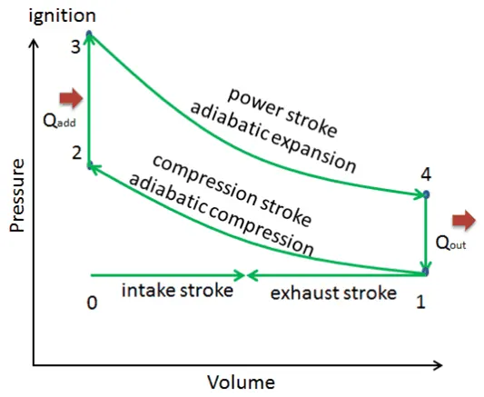
Figure 1: P-V diagram of Otto cycle

• Process 0-1: Suction/Intake Stroke.

A mass of air is drawn into the cylinder at constant pressure. During this process, the intake valve remains open while the exhaust valve remains closed.

• Process 1-2: Isentropic Compression.

This process follows compressing the sucked air by the piston moving from BDC to TDC. Consequently, the pressure increases while the volume decreases and become equal to the clearance volume.

• Process 2-3: Constant Volume Heat Addition.

In this process the heat is added to the air by ignition through a spark plug. Rapid burning of air takes place and pressure and temperature increase linearly as volume remains constant in this process. The piston remains at the TDC.

• Process 3-4: Isentropic Expansion.

This process follows expansion of the combusted air and the piston moves from TDC to BDC. Consequently, the pressure decreases while the volume increases.

• Process 4-1: Constant Volume Heat Rejection.

In this process heat is rejected from the mass of air and the piston remains at BDC.

• Process 1-0: Exhaust Stroke:

In this process the mass of air is released to the atmosphere at constant pressure. The exhaust valve remains open in this process.

Governing Equation: -

Isentropic Process: PV^γ = constant..............(i)

Isochoric Process: P /T = constant..............(ii)

Ideal Gas Equation: PV/T = constant...............(iii)

Compression Ratio: CR = (V_s + V_c)/ V_{c...............(iv)}

Swept Volume: V_s= π/4*D_b*S_{l...........................(v)}

Volume change inside the engine combustion chamber is given by: V = V_c * ( 1 + 1/2 * ( CR - 1)[ R + 1- cosθ - ( R² – sin²θ)^1/2]...........(vi)

Thermal Efficiency of the engine is given by: η = 1 – 1 / (CR-1)^γ *100...........(vii)

Where,

P = Pressure in Pascal

V = Volume inside the cylinder in m³

T = Temperature in Kelvin

CR = Compression Ratio

V_s = Swept Volume

D_b = Cylinder bore diameter in m³

S_l = Stroke length of the piston in m

V_c = Clearance Volume

η = Thermal Efficiency of the engine

R = Ratio of length of the connecting rod to crank pin radius

γ = Ratio of Specific Heats

Solution Procedure:

• In the first step, 'math' and 'matplotlib.pyplot' libraries are imported to perform mathematical operations and plotting of graphs respectively.
• Since Otto cycle is an air standard cycle, γ is taken as 1.4. A variable ‘gamma’ is created and the value of 1.4 is assigned to the variable.
• Initial conditions of the system's pressure and temperature at state point 1 are known; whose values are 101325 Pa and 500K respectively. The variables ‘p1’ and ‘t1’ are created and their values are assigned to them respecctively.
• The maximum temperature is known and a variable ‘t3’ is created and a value of 2300K is assigned to the variable.
• The variables D_b, S_l, con_rod, CR; representing cylinder bore diameter, stroke length of the piston, length of connecting rod, compression ratio respectively, are created and values of 0.20m, 0.4m, 0.25m, 6 are assigned to each of the variables respectively.
• A function “engine_kinematics” is defined with D_b, S_l, con_rod, CR, start_crank, end_crank as the input arguments. This function calculates the volume trace inside a cylinder when the crank moves from BDC to TDC or TDC to BDC using equation (vi).
• Swept volume and the clearance volume are then calculated using equation (iv) and (v) and the values are stored in variables v_s, v_c.
• The volume of state point 1 is calculated by summing up the values of v_s and v_c and the value is stored in v1.
• The other variables for state 2, 3, and 4 are calculated and the values are stored in variables v2, p2, v3, p3, v4, p4 using equations (i) and (iii).
• The ‘for loop’ is employed to calculate pressure trace inside a cylinder when the crank moves from BDC to TDC or TDC to BDC during processes 1-2, 3-4 respectively.
• Thermal efficiency of the engine is calculated using equation (vii).
• Finally the graph between pressure and volume is plotted which represents the Otto cycle.

Python Program

# TO WRITE A PYTHON PROGRAM TO PLOT THE PV DIAGRAM OF THE OTTO CYCLE AND FIND OUT THE THERMAL EFFICIENCY OF THE ENGINE
# SUBMITTED BY IRFAN SUNNY BARUAH ON 02/02/2022.
#====================================================================================
import math
import matplotlib.pyplot as plt
#------------------------------------------------------------------------------------
# Creating variables p1, t1, gamma and t3 and assigning the given values respectively.
p1 = 101325 # Pressure @ state point 1 in Pa.
t1 = 500    # Temperature @ state point 1 in K.
gamma = 1.4 # Ratio of specific heats.
t3 = 2300   # Temperature @ state point 1 in K.
#-----------------------------------------------------------------------------------
# @Engine Geometric Specifications
D_b = 0.20     # Cylinder bore diameter in m.
S_l = 0.4      # Stroke length in m.
con_rod = 0.25 # Length of the connecting rod in m.
CR = 6         # Compression ratio. 
#------------------------------------------------------------------------------------
# Defining a function with D_b, S_l, con_rod, CR, start_crank, end_crank as the input arguments.
def engine_kinematics(D_b, S_l, con_rod, CR, start_crank, end_crank):
	c_p = S_l/2 # Crank Pin Radius.
	R = con_rod/c_p #Ratio of length of the connecting rod to crank pin radius.
	sc = math.radians(start_crank)
	ec = math.radians(end_crank)
	n_theta = 50
	d_theta = (ec-sc)/(n_theta-1)
	V = []
	for i in range(0,n_theta):
		theta = sc+i*d_theta
		term1 = 0.5*(CR-1)
		term2 = R+1-math.cos(theta)
		term3 = pow(pow(R,2) - pow(math.sin(theta),2),0.5)
		V.append(v_c*(1+term1*(term2-term3)))
	return V
#-------------------------------------------------------------------------------------
# Calculating the swept and clearance volume(m^3) of the engine.
v_s = (math.pi/4)*pow(D_b,2)*S_l
v_c = v_s/(CR-1)
#-------------------------------------------------------------------------------------
# @ STATE POINT1: Calculating the volume(m^3) v1.				
v1 = v_c+v_s
#-------------------------------------------------------------------------------------
# @ STATE POINT2: Calculating the variables v2, p2,t2 and pressures for different crank angle when the piston moves from BDC to TDC. 
v2 =v_c  
p2 = p1*pow(v1,gamma)/pow(v2,gamma)
rhs = p1*v1/t1
t2 = p2*v2/rhs
P_comp = []
V_comp = engine_kinematics(D_b, S_l, con_rod, CR, 180, 0)
constant = p1*pow(v1,gamma)
for v in V_comp:
	P_comp.append(constant/pow(v, gamma))
#-------------------------------------------------------------------------------------
# @ STATE POINT2: Calculating the variables v3, p3,t3 and pressures for different crank angle when the piston moves from TDC to BDC. 
v3 =v2
p3 = rhs*t3/v3
P_expan = []
V_expan = engine_kinematics(D_b, S_l, con_rod, CR, 180, 0)
constant = p3*pow(v3,gamma)
for v in V_expan:
	P_expan.append(constant/pow(v, gamma))
#-------------------------------------------------------------------------------------
# @ STATE POINT4: Calculating the variables v4, p4,t4.
v4 =v1
p4 =p3*pow(v3,gamma)/pow(v4, gamma)
t4 = p4*v4/rhs
#-------------------------------------------------------------------------------------
# Thermal Efficiency of the engine
thermal_eff = (1-(1/pow(CR, gamma-1)))*100
print('Thermal efficiency of the engine = {}%'.format(thermal_eff))
#-------------------------------------------------------------------------------------
# PLOTTING OF THE OTTO CYCLE
plt.figure()
plt.grid()
plt.title("Air Standard Otto Cycle", fontname ="Times New Roman", fontsize = 10, fontweight = 'bold')
plt.plot(V_comp,P_comp,color = 'red', linewidth = 1.5, label = "Proc 1-2: Isentropic Compression")
plt.plot([v2,v3],[p2,p3], color = 'black', linewidth = 1.5 ,label = "Proc 2-3:Constant Volume Heat Addition")
plt.plot(V_expan,P_expan, color = 'yellow', linewidth = 1.5, label = "Proc 3-4:Isentropic Expansion")
plt.plot([v1,v4],[p1,p4], color = 'blue', linewidth = 1.5, label ="Proc 4-1:Constant volume heat rejection")
plt.xlabel("Volume in m^3", fontname ="Times New Roman", fontsize = 10, fontweight = 'bold')
plt.ylabel("Pressure in Pa", fontname ="Times New Roman", fontsize = 10, fontweight = 'bold')
plt.plot(v1,p1,'*')
plt.plot(v2,p2,'*')
plt.plot(v3,p3,'*')
plt.plot(v4,p4,'*')
plt.legend()
plt.savefig("Air Standard Otto Cycle")
plt.show()
#=====================================================================================







		

	

Result and Discussion:-

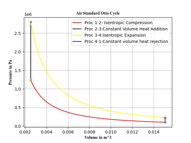
The graph between pressure and volume representing the Otto cycle is plotted and also the thermal efficiency is calculated and are shown below:

1. For compression ratio = 6

2. For compression ratio = 10

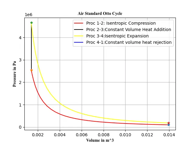
The thermal efficiency of the engine is increasing in the second instance because the compression ratio is higher. The higher the compression ratio, more the air get compressed which leads to the increase in efficiency.