Week 3 - Solving second order ODEs

Objective: - To write a python program to solve the second order differential equation of a simple pendulum to simulate its transient behaviour and to animate the motion of the simple pendulum.

Problem Statement: - ODE is used to describe the transient behaviour of a system. A simple example is a pendulum .The motion of pendulum is governed by Newton’s second law. When this law is written down, we get a second order Ordinary Differential Equation that describes the position of the "ball" w.r.t time. Using, L=1 metre, m=1 kg, b=0.05. g=9.81 m/s2, the motion of a pendulum is to be simulated between 0-20 sec, for angular displacement=0, angular velocity=3 radians/sec at time t=0. Furthermore, the animation of the motion of the pendulum is to be created.

Theory: - A simple pendulum is a mechanical arrangement that demonstrates periodic motion. The simple pendulum comprises a small bob of mass suspended by a thin string secured to a platform at its upper end of length. The simple pendulum is a mechanical system that sways or moves in an oscillatory motion. This motion occurs in a vertical plane and is mainly driven by the gravitational force.

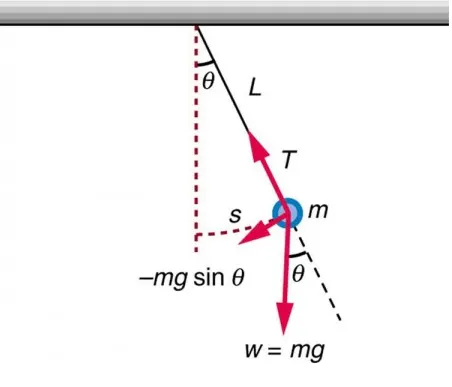
Figure1: Simple Pendulum

Governing Equation: -

The ODE which represents the equation of motion of a simple pendulum with damping is given by:

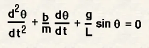
In the above equation,

g = gravity in m/s²

L = length of the pendulum in m,

m = mass of the ball in kg,

b=damping coefficient.

Solution Procedure: -

• The first steps involves breaking down of 2^nd order differential equation into two first order differential equations

Let’s consider θ =θ₁

dθ/dt = dθ₁/dt = θ₂

d² θ/dt² +b/m* dθ/dt + g/L*sinθ =0

dθ₂/dt = -b/m*θ₂ + g/L*sinθ₁

• Numpy, math and matplotlib library are imported to perform array, mathematical operations and to plot graphs respectively.
• From scipy library odeint function is imported to solve the differential equation. The os library is also imported to create a new directory and to join the path of the generated images to the directory for animation of the motion of the pendulum.
• A function named 'model' is defined with theta, t_s, b, g, L, m as the input arguments.
• The inputs b = 0.05, g = 9.81m/s², L = 1m, m = 1kg for simple pendulum were given to the IDE.
• The initial conditions for angular displacement and velocity which is given as 0 and 3 rad/sec are defined. A variable t_s is created to store the value of time period from 0 to 20 seconds.
• A variable theta is created for storing the values of ODE. The function 'odeint' is called for solving the ODE.
• Finally the graph of damped harmonic motion of the simple pendulum is plotted.
• For the animation of the simple pendulum a folder name Pendulum is created using os.mkdir function.
• Using a counter variable ct and for loop the plots are generated and saved in the created directory using the os.path.join() function. Finally, ImageMagick is employed to create the animation of the motion of the simple pendulum.

Python Program:-

# TO WRITE A PYTHON PROGRAM TO SOLVE THE ODE REPRESENTING THE EQUATION OF MOTION OF A PENDULUM AND SIMULATE ITS MOTION.
# SUBMITTED BY IRFAN SUNNY BARUAH ON 05/02/2022.
#=======================================================================================================================
import numpy as np
import math
import matplotlib.pyplot as plt
from scipy.integrate import odeint
import os
#-----------------------------------------------------------------------------------------------------------------------
# Defining a function named 'model' with theta, t_s, b, g, L, m as the input arguments.
def model(theta, t_s, b, g, L, m):

	theta1 = theta[0]
	theta2 = theta[1]
	dtheta1_dt = theta2
	dtheta2_dt = -(b/m)*theta2-(g/L)*math.sin(theta1)
	dtheta_dt =[dtheta1_dt, dtheta2_dt]
	return dtheta_dt
#-----------------------------------------------------------------------------------------------------------------------
# Inputs for simple pendulum.
b = 0.05    # Damping coefficient.
g = 9.81    # Acceleration due to gravity in m/s^2.
L = 1       # Length of the string in m.
m = 1       # Mass of the ball in kg.
#-----------------------------------------------------------------------------------------------------------------------
# Defining the initial conditions for angular displacement and velocity which is given as 0 and 3 rad/sec.
theta_0 = [0, 3]
# Creating a variable t_s to store the value of time period from 0 to 20 seconds.
t_s = np.linspace(0,20,150)
#-----------------------------------------------------------------------------------------------------------------------
# Creating a variable theta and storing the values of ODE solved by using function 'odeint'
theta = odeint(model,theta_0,t_s,args =(b,g,L,m))
#-----------------------------------------------------------------------------------------------------------------------
# Plotting of the Damped Harmonic motion of the Simple Pendulum. 
plt.figure()
plt.grid()
plt.plot(t_s, theta[:,0],'k-',label= r'$\frac{d\theta_1}{dt} = \theta_2$')
plt.plot(t_s, theta[:,1],'r--',label= r'$\frac{d\theta_2}{dt} = -\frac{b}{m}-\frac{g}{L}*sin\theta_1$')
plt.legend(loc = 'best',fontsize= 10)
plt.xlabel('Time Period(seconds)',fontname ="Times New Roman", fontsize = 10, fontweight = 'bold')
plt.ylabel('Angular Displacement(rad) and Velocity(rad/sec)',fontname ="Times New Roman", fontsize = 10, fontweight = 'bold')
plt.title('Harmonic Motion of a Damped Simple Pendulum',fontname ="Times New Roman", fontsize = 10, fontweight = 'bold')
plt.savefig('Damped Simple Pendulum')
plt.show()
#------------------------------------------------------------------------------------------------------------------------
# Animation of the Simple Pendulum.
folder_name = "Pendulum"
os.mkdir(folder_name)
ct = 1
tmp = theta[:,0]
for i in range(len(t_s)):
	x_start = 0
	y_start = 0
	x_end = L*math.sin(tmp[i])
	y_end = -L*math.cos(tmp[i])
	filename = 'Pendulum%05d.png'%ct
	plt.figure()
	plt.grid()
	plt.plot([x_start, x_end],[y_start,y_end], linewidth =3,color ='green')     # Plotting the string of the pendulum.
	plt.plot(x_end,y_end,'o', markersize = 20, color ='pink')     # Plotting the bob of the pendulum.
	plt.plot([0,0],[0,-1.25],'--', color = 'grey', linewidth = 2) # Plotting of vertical reference line -ve y-axis.
	plt.plot([0,0],[0,1.25],'--', color = 'grey', linewidth = 2)  # Plotting of vertical reference line +ve y-axis.
	plt.plot([-1, 1],[0,0], linewidth = 8,color ='yellow')        # Plotting of the rigid support suspending the pendulum.
	plt.title('Harmonic Motion of a Damped Simple Pendulum',fontname ="Times New Roman", fontsize = 10, fontweight = 'bold')
	plt.xlim([-1.5,1.5])
	plt.ylim([-1.5,1.5])
	plt.savefig(os.path.join(folder_name, filename))
	ct = ct + 1
#=================================================================================================================================

Result and Discussion:-

The graph for damped harmonic motion of the simple pedulum is plotted as shown below:

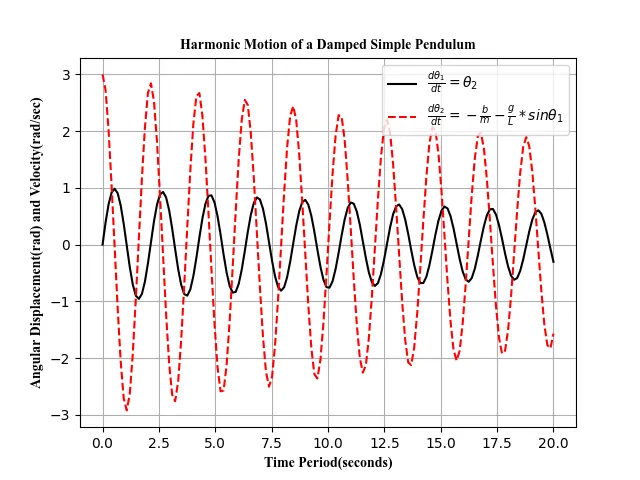
Figure2: Damped Harmonic Motion of a Simple Pendulum

ImageMagick is used and the animation is created and provided in the link below:

https://drive.google.com/drive/folders/1dih070u7IqqprBEa3pjS1I-SOkQdDTG-?usp=sharing