Week 5 - Curve fitting
AIM:
To explain some concepts
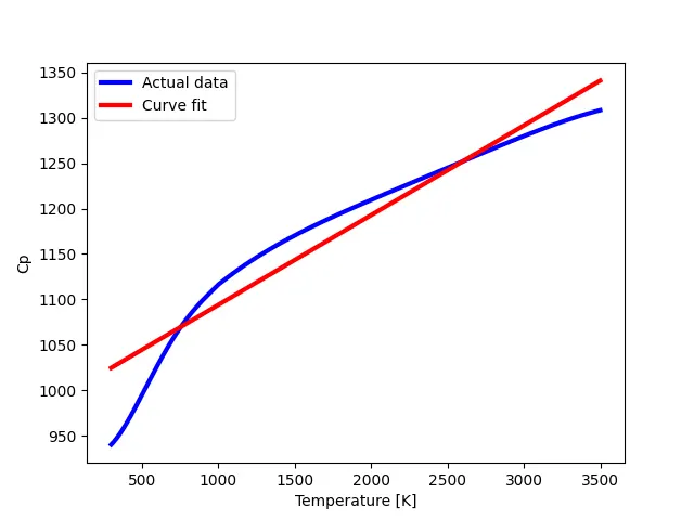
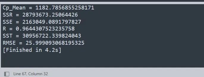
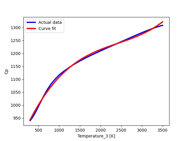
To write code to fit a linear and cubic polynomial for the Cp data and explain if your results are good or bad.
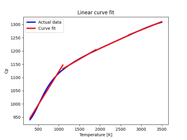
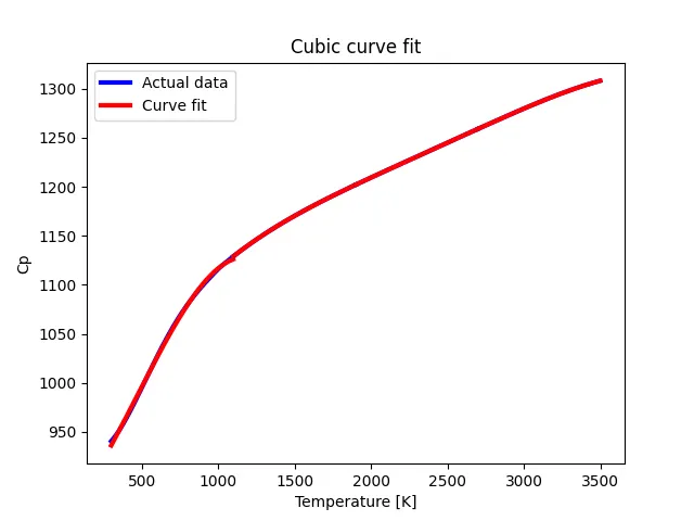
Plot the linear and cubic fit curves along with the raw data points. Title and axes labels are a must, legends could be shown if necessary
Write a code to show splitwise method
LANGUAGE: Python
Editor : Sublime Text
SUMMARY:
Concepts & Definition
Code and explanation
Conclusion
References
Concepts & Definition
Curve fitting is the process of constructing a curve, or mathematical function, that has the best fit to a series of data points, possibly subject to constraints. In order other words Polynomial curve fitting is when we fit our data to the graph of a polynomial function. The same least squares method can be used to find the polynomial, of a given degree, that has a minimum total error.
Fitted curves can be used as an aid for data visualization, to infer values of a function where no data are available, and to summarize the relationships among two or more variables.
Concepts related to python
popt:
It is the first output argument when calling the fitting function. 'popt' is an array which consists the optimal (best fit) values of coefficients of a polynomial, used for curve fitting process, for which the sum of squared residuals for a given data is minimized.
pcov :
It is the second output argument. 'pcov' is a 2D array which gives an estimated values of covariance of coefficients (popt) of a polynomial. The diagonal elements of an array/matrix gives the value of covariance of a coefficient with itself which is also called as variance of that coefficent. Other non-diagonal elements of the matrix gives the covariance of a coefficient with other coefficient. It is a square matrix (no. of rows = no. of columns). This array/matrix indicates the uncertainities and correlation between the coefficients of a polynomial and it is mostly useful when the data has uncertainities. 'pcov' can be used to find the standard deviation (square root of the value of diagonal elements) of a given dataset.
* in *popt mean:
The star i.e '*' in '*popt' unpacks the 'popt' array so that the optimized coefficients (parameters) values can be accessed from the array 'popt'. In other words, '*' aids in referring to all the values stored in the array 'popt'.
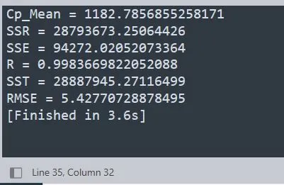
Explanation of the parameters used to measure the fitness characteristics for both the curves.
Let’s assume f(x) is the function that fit well the given that set
Let’s say the function is first degree function
So f(x)=ax+b where the a & b are the coefficients
If the degree of the function is increasing, Obviously the number of coefficient also increases
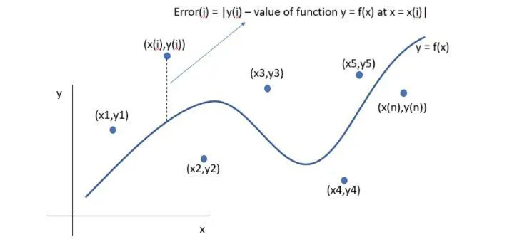
The error for a general 'i' point can be can be given by:
Error=|y(i)−f(x(i))|
Calculation of sum of square of regression
SSR=∑((f(x(i))−Mean)^2 (for i = 1 to n)
Calculation of sum of squared errors(SSE)
SSE=∑(y(i)−f(x(i)))^2 (for i = 1 to n)
SST is given by:
SST=SSR+SSE
Hence R2=SSR/SST
where SSR is Sum of squares of the regression which is the the square of the difference between the value of the fitting function at a given point and the arithmetic mean of the data set.
Calculation of root mean square of error
RMSE=(SSE/n)^0.5
where n is the total number of dataset points available
Code and explanation
Using linear fitting polynomial
"""
Code to perform splitwise method for curve fitting uding linear and cubic polynomials

"""

#Importing the required libraries
import numpy as np
import matplotlib.pyplot as plt
from scipy.optimize import curve_fit

# Curve fit function
def func(t, a, b):
	return a*t + b

#Reading thermodynamic data  file
def read_file():
	temperature = []
	cp = []
	for line in open('data','r'):
		values = line.split(',')
		temperature.append(float(values[0]))
		cp.append(float(values[1]))

	return [temperature, cp]

#Main program

#Reading the file and recording data in variables
temperature, cp = read_file()

#Calculation of the coffecients of linear fitting polynomial
popt, pcov = curve_fit(func, temperature, cp)
fit_cp = func(np.array(temperature), *popt)

plt.plot(temperature, cp,color="blue",linewidth=3)
plt.plot(temperature, fit_cp,color="red",linewidth=3)
plt.legend(['Actual data','Curve fit'])
plt.xlabel('Temperature [K]')
plt.ylabel('Cp')

plt.show()

#For Cubic fitting

#Calculation of the mean
sum_1=0 #initialization
for i in range(0,len(cp)) :
	sum_1=sum_1 + cp[i]

mean=sum_1/len(cp)
print('Cp_Mean =',mean)

#Calculation of the value of SSR, SSE, SST
#Initialization
SSE_1=0
SSR_1=0

for i in range (0, len(cp)):
    SSR_1=SSR_1 + pow(cp[i]-mean,2)

for i in range (0, len(cp)):
    SSE_1 = SSE_1 + pow(fit_cp[i]-cp[i],2)


SST_1 = SSR_1 + SSE_1
R1 = pow(SSR_1/SST_1,0.5)
RMSE_1 = pow(SSE_1/len(cp),0.5)


print('SSR =',SSR_1)
print('SSE =',SSE_1)
print('R =',R1)
print('SST =',SST_1)
print('RMSE =',RMSE_1)
Output
Using cubic fitting polynomial
"""
Code to perform splitwise method for curve fitting uding linear and cubic polynomials

"""

#Importing the required libraries
import numpy as np
import matplotlib.pyplot as plt
from scipy.optimize import curve_fit

# Curve fit function
def func(t, e, f, g, h):
	return e*pow(t,3) + f*pow(t,2) + g*t + h

#Reading thermodynamic data  file
def read_file():
	Temperature_3 = []
	cp = []
	for line in open('data','r'):
		values = line.split(',')
		Temperature_3.append(float(values[0]))
		cp.append(float(values[1]))

	return [Temperature_3, cp]

#Main program
Temperature_3, cp = read_file()
popt, pcov = curve_fit(func, Temperature_3, cp)
fit_cp = func(np.array(Temperature_3), *popt)

#Ploting of the actual and linear fitting curve
plt.plot(Temperature_3, cp,color="blue",linewidth=3)
plt.plot(Temperature_3, fit_cp,color="red",linewidth=3)
plt.legend(['Actual data','Curve fit'])
plt.xlabel('Temperature_3 [K]')
plt.ylabel('Cp')

plt.show()

#For Cubic fitting

#Calculation of the mean
sum_1=0 #initialization
for i in range(0,len(cp)) :
	sum_1=sum_1 + cp[i]

mean=sum_1/len(cp)
print('Cp_Mean =',mean)

#Calculation of the value of SSR, SSE, SST
#Initialization
SSE_1=0
SSR_1=0

for i in range (0, len(cp)):
    SSR_1=SSR_1 + pow(cp[i]-mean,2)

for i in range (0, len(cp)):
    SSE_1 = SSE_1 + pow(fit_cp[i]-cp[i],2)


SST_1 = SSR_1 + SSE_1
R1 = pow(SSR_1/SST_1,0.5)
RMSE_1 = pow(SSE_1/len(cp),0.5)


print('SSR =',SSR_1)
print('SSE =',SSE_1)
print('R =',R1)
print('SST =',SST_1)
print('RMSE =',RMSE_1)
Output
For splitwise method:
"""
Code to perform splitwise method for curve fitting uding linear and cubic polynomials

"""

#Importing the required libraries
import numpy as np
import matplotlib.pyplot as plt
from scipy.optimize import curve_fit

#Linear fitting function
def func1(t, a, b):
	return a*t + b
#cubic fitting function
def func3(t, a, b, c, d):
	return a*pow(t,3) + b*pow(t,2) + c*t + d

#Reading thermodynamic data  file
def read_file():
	temperature = []
	cp = []
	for line in open('data','r'):
		values = line.split(',')
		temperature.append(float(values[0]))
		cp.append(float(values[1]))

	return [temperature, cp]

#Main program

#Reading the file and recording data in variables
temperature, cp = read_file()


#Splitting  the temperature and cp arrays in ranges

temp1 = temperature[1:800]
cp1 = cp[1:800]

temp2 = temperature[801:1600]
cp2 = cp[801:1600]

temp3 = temperature[1601:2400]
cp3 = cp[1601:2400]

temp4 = temperature[2401:3200]
cp4 = cp[2401:3200]

#Calculation of the coffecients of linear fitting polynomial for different ranges
popt11, pcov11 = curve_fit(func1, temp1, cp1)
popt12, pcov2 = curve_fit(func1, temp2, cp2)
popt13, pcov3 = curve_fit(func1, temp3, cp3)
popt14, pcov4 = curve_fit(func1, temp4, cp4)

fit_cp11 = func1(np.array(temp1), *popt11)
fit_cp12 = func1(np.array(temp2), *popt12)
fit_cp13 = func1(np.array(temp3), *popt13)
fit_cp14 = func1(np.array(temp4), *popt14)

#Ploting of the actual and linear fitting curve
plt.figure(1)
plt.plot(temp1, cp1,color="blue",linewidth=3)
plt.plot(temp1, fit_cp11,color="red",linewidth=3)
plt.plot(temp2, cp2,color="blue",linewidth=3)
plt.plot(temp2, fit_cp12,color="red",linewidth=3)
plt.plot(temp3,  cp3,color="blue",linewidth=3)
plt.plot(temp3,  fit_cp13,color="red",linewidth=3)
plt.plot(temp4, cp4,color="blue",linewidth=3)
plt.plot(temp4, fit_cp14,color="red",linewidth=3)
plt.legend(['Actual data','Curve fit'])
plt.xlabel('Temperature [K]')
plt.ylabel('Cp')

plt.show()


#Calculation of the coffecients of cubic fitting polynomial for different ranges

popt31, pcov31 = curve_fit(func3, temp1, cp1)
popt32, pcov32 = curve_fit(func3, temp2, cp2)
popt33, pcov33 = curve_fit(func3, temp3, cp3)
popt34, pcov34 = curve_fit(func3, temp4, cp4)

fit_cp31 = func3(np.array(temp1), *popt31)
fit_cp32 = func3(np.array(temp2), *popt32)
fit_cp33 = func3(np.array(temp3) , *popt33)
fit_cp34 = func3(np.array(temp4), *popt34)

#Ploting of the actual and cubic fitting curve
plt.figure(2)
plt.plot(temp1, cp1,color="blue",linewidth=3)
plt.plot(temp1, fit_cp31,color="red",linewidth=3)
plt.plot(temp2, cp2,color="blue",linewidth=3)
plt.plot(temp2, fit_cp32,color="red",linewidth=3)
plt.plot(temp3,  cp3,color="blue",linewidth=3)
plt.plot(temp3,  fit_cp33,color="red",linewidth=3)
plt.plot(temp4, cp4,color="blue",linewidth=3)
plt.plot(temp4, fit_cp34,color="red",linewidth=3)
plt.legend(['Actual data','Curve fit'])
plt.xlabel('Temperature [K]')
plt.ylabel('Cp')

plt.show()
Output
Conclusion:
To sum up Curve fitting is one of the most powerful and most widely used analysis tools. By splitwise method we can clearly see that the fitting is better and this can be also confirmed by the the parameters used to measure the fitness characteristics. In order to make the curve fit perfect we can increase the degree of the fitting polynomial or use the splitwise polynomial method.
References:
https://en.wikipedia.org/wiki/Curve_fitting
https://docs.scipy.org/doc/scipy/reference/generated/scipy.optimize.curve_fit.html