Project 2 - Rankine cycle Simulator

Project: Rankine cycle Simulator

Aim: To create a Rankine Cycle Simulator using MATLAB.

LANGUAGE: Matlab

SOFTWARE: Matlab R2019a

SUMMARY:

Objective

Theory & Definition

Code and explanation

Conclusion

References

Objective:

To write a code to calculate the state points of the Rankine Cycle based on user inputs.

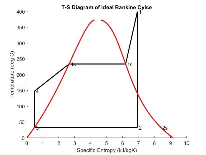
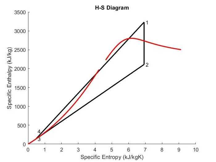
To plot the corresponding T-s and h-s plots for the given set of inputs

Theory & Definition:

The Rankine cycle is the fundamental operating cycle of all power plants where an operating fluid is continuously evaporated and condensed. In this mechanism, a fuel is used to produce heat within a boiler, converting water into steam which then expands through a turbine producing useful work. This is a thermodynamic cycle which converts heat into mechanical energy which usually gets transformed into electricity by electrical generation. The Rankine cycle or Rankine Vapor Cycle is the process widely used by power plants such as coal-fired power plants or nuclear reactors. This process was developed in 1859 by Scottish engineer William J.M. Rankine.

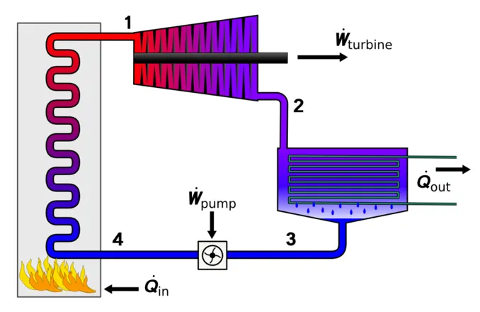
The main components of a rankine cycle are:

Pump: Used to compress the fluid to high pressure (this takes work).

`h_f3+W_p=h_f4`

Where `W_p=` pump work

`W_p=h_f4-h_f3`

Boiler: The compressed fluid is heated to the final temperature (which is at boiling point), therefore, a phase change occurs—from liquid to vapor.

Turbine: Expansion of the vapor occurs in the turbine.

`h_1=W_T+h_2`

Where `W_T` is turbine work

`W_T=h_1-h_2`

Condenser: Condensation of the vapor in the condenser (where the waste heat goes to the final heat sink (the atmosphere or a large body of water.

`h_2=Q_(out)+h_f3`

`Q_(out)=h_2-h_f3`

Efficiency of Rankine cycle is given by:

`Eff_(Rank.)=(W_(n))/(Q_(i))=(W_T-W_T)/Q_(i)`

Where `Q_i` is the incoming heat energy from the boiler

1-2 Isentropic Expansion. The vapor is expanded in the turbine, thus producing work which may be converted to electricity. In practice, the expansion is limited by the temperature of the cooling medium and by the erosion of the turbine blades by liquid entrainment in the vapor stream as the process moves further into the two-phase region. Exit vapor qualities should be greater than 90% to increase the life of turbine blade.

2-3 Isobaric Heat Rejection. The vapor-liquid mixture leaving the turbine is condensed at low pressure, usually in a surface condenser using cooling water. In well designed and maintained condensers, the pressure of the vapor is well below atmospheric pressure, approaching the saturation pressure of the operating fluid at the cooling water temperature.

3-4 Isentropic Compression. The pressure of the condensate is raised in the feed pump. Because of the low specific volume of liquids, the pump work is relatively small and often neglected in thermodynamic calculations.

4-1 Isobaric Heat Transfer. High pressure liquid enters the boiler from the feed pump and is heated to the saturation temperature. Further addition of energy causes evaporation of the liquid until it is fully converted to saturated steam.

Required Inputs:

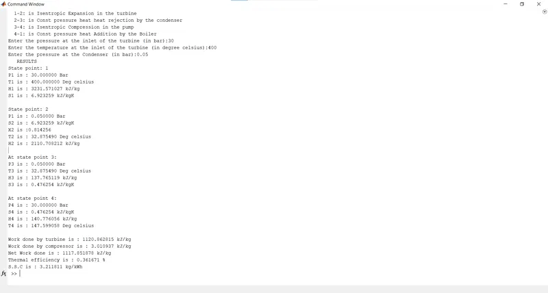
Turbine Inlet temperature = 400° C

Turbine Inlet Pressure = 30 bars

Turbine Outlet Pressure = 0.05 bars = Condenser Inlet Pressure

Code and explanation:

clear all
close all
clc
fprintf('  1-2: is Isentropic Expansion in the turbine \n');
fprintf('  2-3: is Const pressure heat heat rejection by the condenser\n');
fprintf('  3-4: is Isentropic Compression in the pump \n');
fprintf('  4-1: is Const pressure heat Addition by the Boiler\n');

P1=input('Enter the pressure at the inlet of the turbine (in bar):');
T1=input('Enter the temperature at the inlet of the turbine (in degree celsius):');

P2=input('Enter the pressure at the Condenser (in bar):');

disp('   RESULTS')
%Let's get Cp and cv values from Xsteam 
%We assumed that Cp and Cv do not change with temperature to make problem simple

% for vapour
HIGH_cpV= XSteam('CpV_p', P1);
LOW_cpV=XSteam('CpV_p', P2);
HIGH_cvV=XSteam('CvV_p', P1);
LOW_cvV=XSteam('CvV_p', P2);

% for liquid
HIGH_cpL= XSteam('CpL_p', P1);
LOW_cpL=XSteam('CpL_p', P2);
HIGH_cvL=XSteam('CvL_p', P1);
LOW_cvL=XSteam('CvL_p', P2);

%Getting important parameters from Xsteam 
%for high pressure
T1s = XSteam('Tsat_p', P1);
S1g = XSteam('sV_p', P1);
S1f = XSteam('SL_p', P1);
S1fg = S1g - S1f;
H1f = XSteam('hL_p', P1);
H1g = XSteam('hV_p', P1);
H1fg = H1g - H1f;
%for low pressure
S2g = XSteam('sV_p', P2);
S2f = XSteam('SL_p', P2);
S2fg = S2g - S2f;
T2s = XSteam('Tsat_p', P2);
H2f = XSteam('hL_p', P2);
H2g = XSteam('hV_p', P2);
H2fg = H2g - H2f;

% State point 1
disp('State point: 1')
fprintf('P1 is : %f Bar \n', P1)
fprintf('T1 is : %f Deg celsius \n', T1)

H1 = XSteam('h_pt', P1, T1);
fprintf('H1 is : %f kJ/kg \n', H1)

S1 = XSteam('s_pt', P1, T1);
fprintf('S1 is : %f kJ/kgK \n', S1)
fprintf('\n')

% State point 2
disp('State point: 2')
fprintf('P1 is : %f Bar \n', P2) %we already input P2
S2 = S1;
fprintf('S2 is : %f kJ/kgK \n', S2)
%Let's predict the location of point 2 in T-s diagram
if(S2<=S2g)
    X2 = (S2 - S2f) / (S2fg);   % Dryness Fraction at state point 2
else
    X2=1;    
end

fprintf('X2 is :%f \n', X2)

%Let's calculate T2 for superheat or wet or dry wherever it lies:
if(X2<1)
    T2=T2s;
else 
    %t2 called by s2=s2g+LOW_cpV*(log(T2/T2s))
    T2=(T2s+273.15)*exp((S2-S2g)/LOW_cpV) ; %2 in superheated region
    T2=T2-273.15;
end    
fprintf('T2 is : %f Deg celsius \n', T2)

if(X2<1)
   H2 = H2f + X2 * H2fg;
else
   H2=H2g+ LOW_cpV*(T2-T2s); 
end   
fprintf('H2 is : %f kJ/kg \n', H2)
fprintf('\n')

% State point 3
%Let's assume no subcooling in the condenser
disp('At state point 3:')
P3 = P2;
fprintf('P3 is : %f Bar \n', P3)
V3 = XSteam('vL_p', P3);
T3 = T2s;    %no subcooling assumed
fprintf('T3 is : %f Deg celsius \n', T3)
H3 =H2f;
fprintf('H3 is : %f kJ/kg \n', H3)
S3 =S2f;
fprintf('S3 is : %f kJ/kgK \n', S3)
fprintf('\n')
% State point 4
disp('At state point 4:')
P4 = P1;
fprintf('P4 is : %f Bar \n', P4)

S4 = S3;
fprintf('S4 is : %f kJ/kgK \n', S4)
Wp = V3 * (P4 - P3) * 100;
H4 = Wp + H3;
fprintf('H4 is : %f kJ/kg \n', H4)
% Let's  cal T4; s4=s3=sf1-HIGH_cpL*ln(t1s/t4)
term=exp((S1f-S4)/HIGH_cpL);  %Use exp instead of Exp to take input as double
T4= T1s/term;
fprintf('T4 is : %f Deg celsius \n', T4)
fprintf('\n')

%Let's calculate Work done, heat, SSC and efficiency
Wt = H1 - H2;
fprintf('Work done by turbine is : %f kJ/kg \n', Wt)
fprintf('Work done by compressor is : %f kJ/kg \n', Wp)
Wnet = Wt - Wp;
fprintf('Net Work done is : %f kJ/kg \n', Wnet)
Qin = H1 - H4;
Thermal_eff = Wnet / Qin ;    % Efficiency
fprintf('Thermal efficiency is : %f ', Thermal_eff); 
disp('%')
SSC = 3600 / Wt;    % Specific steam consumption
fprintf('S.S.C is : %f kg/kWh \n ', SSC)
%Let's calculate data for plotting Liquid and Vapour lines:
temp = linspace(1, 373, 500);
for i = 1 : length(temp)
     H_L(i) = XSteam('hL_T', temp(i));
     H_V(i) = XSteam('hV_T', temp(i));
     S_L(i) = XSteam('sL_T', temp(i));
     S_V(i) = XSteam('sV_T', temp(i));
end

%Let's plot T-S and H-S Diagrams :
% T-S plotting
figure(1) % T-S diagram
hold on %to hold on
%PLOTTING & PHASES MENTION
plot([S1 S2], [T1 T2s], 'k', 'linewidth', 2)
text(S1,T1,' 1')
text(S2,T2s,' 2')
text(S2g,T2s,' 2s')
plot([S3 S2], [T2s T3], 'k', 'linewidth', 2)
text(S3,T3,' 3')
plot([S3 S4], [T3 T4], 'k', 'linewidth', 2)
text(S4,T4,' 4')
plot([S4 S1f], [T4 T1s], 'k', 'linewidth', 2)
text(S1f,T1s,' 4s')
plot([S1f S1g], [T1s T1s], 'k', 'linewidth', 2)
text(S1g,T1s,' 1s')
plot([S1g S1], [T1s T1], 'k', 'linewidth', 2)
plot(S_L, temp, 'r','linewidth', 2)
plot(S_V, temp, 'r','linewidth', 2)
%titling
title('T-S Diagram of Ideal Rankine Cylce')
%labelling
ylabel('Temprature (deg C)')
xlabel('Specific Entropy (kJ/kgK)')

% H-S Plotting
figure(2) 
hold on %to hold on 
%PLOTTING & PHASES MENTION
plot([S1 S2], [H1 H2], 'k', 'linewidth', 2);
text(S1,H1,' 1')
plot([S2 S3], [H2 H3], 'k', 'linewidth', 2);
text(S2,H2,' 2')
plot([S3 S4], [H3 H4], 'k', 'linewidth', 2);
text(S3,H3,' 3')
plot([S4 S1], [H4 H1], 'k', 'linewidth', 2);
text(S4,H4+200,' 4')
plot(S_L, H_L, 'r','linewidth',2)
plot(S_V, H_V, 'r','linewidth',2)      
title('H-S Diagram')
ylabel('Specific Enthalpy (kJ/kg)')
xlabel('Specific Entropy (kJ/kgK)')

Output:

Conclusion:

As rankine cycle is an idealized thermodynamic cycle describing the process by which certain heat engines allow mechanical work to be extracted from a fluid, we can modify it as needed according to the conditions but the principle remains the same.

References:

https://energyeducation.ca/encyclopedia/Rankine_cycle

https://thermopedia.com/content/1072

https://www.mathworks.com/help/matlab/ref/plot.html

https://www.mathworks.com/help/matlab/creating_plots/using-high-level-plotting-functions.html