Week 4.1 - Genetic Algorithm
AIM:
To write a code in MATLAB to optimise the stalagmite function and find the global maxima of the function.
To expalin the concept of genetic algorithm in your own words and also explain the syntax for ga in MATLAB in your report.
To plot graphs for all 3 studies and for F maximum vs no. of iterations.
LANGUAGE: Matlab
SOFTWARE: Matlab R2019a
SUMMARY:
Theory & Definition
Code and explanation
Conclusion
References
Theory & Definition
A stalagmite is a type of speleothem that rises from the floor of a limestone cave due to the dripping of mineralized solutions and the deposition of calcium carbonate.
A stalagmite function refers to the function used for generating values over a stalagmite kind of surface for finding out the local and global maxima and minima of that particular given function.
A genetic algorithm is a search heuristic that is inspired by Charles Darwin’s theory of natural evolution. This algorithm reflects the process of natural selection where the fittest individuals are selected for reproduction in order to produce offspring of the next generation.
It is used to find optimal and near-optimal solutions to complex problems which could normally take a lifetime to be solved. Precisely it is used in optimization problems and machine learning.
Syntax of genetic algorithm:
x = ga(fun,nvars)
x = ga(fun,nvars,A,b)
x = ga(fun,nvars,A,b,Aeq,beq)
x = ga(fun,nvars,A,b,Aeq,beq,lb,ub)
x = ga(fun,nvars,A,b,Aeq,beq,lb,ub,nonlcon)
x = ga(fun,nvars,A,b,Aeq,beq,lb,ub,nonlcon,options)
x = ga(fun,nvars,A,b,[],[],lb,ub,nonlcon,IntCon)
x = ga(fun,nvars,A,b,[],[],lb,ub,nonlcon,IntCon,options)
x = ga(problem)
[x,fval] = ga(___)
[x,fval,exitflag,output] = ga(___)
[x,fval,exitflag,output,population,scores] = ga(___)
Explanation of the syntax:
x = ga(fun,nvars) finds a local unconstrained minimum, x, to the objective function, fun. nvars is the dimension (number of design variables) of fun.
x = ga(fun,nvars,A,b) finds a local minimum x to fun, subject to the linear inequalities A*x ≤ b. ga evaluates the matrix product A*x as if x is transposed (A*x').
x = ga(fun,nvars,A,b,Aeq,beq) finds a local minimum x to fun, subject to the linear equalities Aeq*x = beq and A*x ≤ b. (Set A=[] and b=[] if no linear inequalities exist.) ga evaluates the matrix product Aeq*x as if x is transposed (Aeq*x').
x = ga(fun,nvars,A,b,Aeq,beq,lb,ub) defines a set of lower and upper bounds on the design variables, x, so that a solution is found in the range lb ≤ x ≤ ub. (Set Aeq=[] and beq=[] if no linear equalities exist.)
x = ga(fun,nvars,A,b,Aeq,beq,lb,ub,nonlcon) subjects the minimization to the constraints defined in nonlcon. The function nonlcon accepts x and returns vectors C and Ceq, representing the nonlinear inequalities and equalities respectively. ga minimizes the fun such that C(x) ≤ 0 and Ceq(x) = 0. (Set lb=[] and ub=[] if no bounds exist.)
x = ga(fun,nvars,A,b,Aeq,beq,lb,ub,nonlcon,options) minimizes with the default optimization parameters replaced by values in options. (Set nonlcon=[] if no nonlinear constraints exist.) Create options using optimoptions.
x = ga(fun,nvars,A,b,[],[],lb,ub,nonlcon,IntCon) or x = ga(fun,nvars,A,b,[],[],lb,ub,nonlcon,IntCon,options) requires that the variables listed in IntCon take integer values.
x = ga(problem) finds the minimum for problem, a structure described in problem.
[x,fval] = ga(___), for any previous input arguments, also returns fval, the value of the fitness function at x.
[x,fval,exitflag,output] = ga(___) also returns exitflag, an integer identifying the reason the algorithm terminated, and output, a structure that contains output from each generation and other information about the performance of the algorithm.
[x,fval,exitflag,output,population,scores] = ga(___) also returns a matrix population, whose rows are the final population, and a vector scores, the scores of the final population.
5 phases are considered in genetic algorithm:
Initial Population
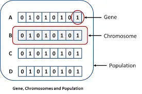
The process begins with a set of individuals which is called a Population. Each individual is a solution to the problem you want to solve. An individual is characterized by a set of parameters (variables) known as Genes. Genes are joined into a string to form a Chromosome (solution).
Selection
The idea of selection phase is to select the fittest individuals and let them pass their genes to the next generation
Two pairs of individuals (parents) are selected by considering their fitness scores. Therefore individuals with high fitness have more chance to be selected for reproduction.
Fitness Function
The fitness function shows how fit an individual is (the ability of an individual to compete with other individuals). It gives a fitness score to each individual. The probability that an individual will be selected as a parent for reproduction is based on its fitness score.
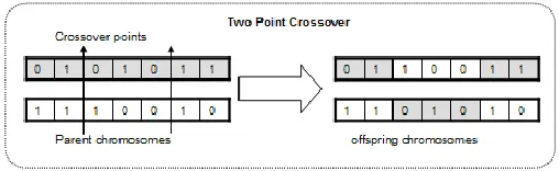
Crossover: Also called recombination, is a genetic operator used to combine the genetic information of two parents to generate new offspring. It is one way to stochastically (randomly) generate new solutions from an existing population, and is analogous to the crossover that happens during sexual reproduction in biology.
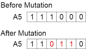
Mutation, analogous to biological mutation is a genetic operator used to maintain genetic diversity from one generation of a population of genetic algorithm chromosomes to the next. Mutation alters one or more gene values in a chromosome from its initial state. In mutation, the solution may change entirely from the previous solution. Hence GA can come to a better solution by using mutation. Mutation occurs during evolution according to a user-definable mutation probability. This probability should be set low. If it is set too high, the search will turn into a primitive random search.
Code and explanation
Function:
%stalagmite function
function Sta=stalagmite(input_vector)
x=input_vector(1);
y=input_vector(2);
f1=(sin(5.1*pi*x+0.5))^6;
f2=(sin(5.1*pi*y+0.5))^6;
f3=exp(-4*log(2)*(((x-0.0667)^2)/0.64));
f4=exp(-4*log(2)*(((y-0.0667)^2)/0.64));
Sta=-f1*f2*f3*f4;
end
Main code:
close all %to clear the previous work data
clear all % to close the previous work graphs
clc % to clear the previous work command

% Define your search space
x=linspace(0,0.6,150);
y=linspace(0,0.6,150);
total=30;

% Creating a  2Dimensional mesh
[xx yy]=meshgrid(x,y);
%Evaluating the stalagmite function
for i=1:length(xx)
    for j=1:length(yy)
        input_vector(1)=xx(i,j);
        input_vector(2)=yy(i,j);
        f(i,j)=stalagmite(input_vector);
    end

end

%case1:Unbounded case
tic
for i=1:total

 [inputs,fval(i)]=ga(@stalagmite,2);
 x_out(i)=inputs(1);
 y_out(i)=inputs(2);
end
case1=toc

figure(1)
subplot(2,1,1) % to divide the current figure into an 2-by-1 grid and create axes in the position specified by 1
surfc(xx,yy,-f) %to create the contour plot
shading interp % to remove the strie from the contour plot
xlabel('x_axis')
ylabel('y_axis')
title('Unbounded case')
hold on;
plot3(x_out,y_out,-fval,'marker','o','markersize',6,'markerfacecolor','r')
subplot(2,1,2)
plot(-fval);
xlabel('no of iteration ')
ylabel('max function value')

%case2:bounding box case
tic
for i=1:total

 [inputs,fval(i)]=ga(@stalagmite,2,[],[],[],[],[0,0],[0.6,0.6]);
 x_out(i)=inputs(1);
 y_out(i)=inputs(2);
end
case2=toc

figure(2)
subplot(2,1,1)
hold on;
surfc(xx,yy,-f)%to create the contour plot
shading interp %to remove the strie from the contour plot
xlabel('x_axis')
ylabel('y_axis')
title('case 2: with Bounding Box')
hold on;
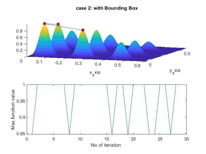
plot3(x_out,y_out,-fval,'marker','o','markersize',6,'markerfacecolor','r')
subplot(2,1,2)
plot(-fval);
xlabel('No of iteration ')
ylabel('Max function value')


%case3:
options=optimoptions('ga');
options=optimoptions(options,'populationsize',100);

tic
for i=1:total

 [inputs,fval(i)]=ga(@stalagmite,2,[],[],[],[],[0,0],[0.6,0.6],[],[],options);
 x_out(i)=inputs(1);
 y_out(i)=inputs(2);
end
case3=toc

figure(3)
subplot(2,1,1)
hold on;
surfc(xx,yy,-f) %to create the contour plot
shading interp %to remove the strie from the contour plot
xlabel('x_axis')
ylabel('y_axis')
title(' case 3: Bounded with increased population size')
hold on;
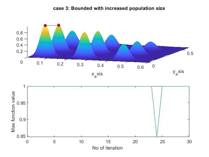
plot3(x_out,y_out,-fval,'marker','o','markersize',6,'markerfacecolor','r')
subplot(2,1,2)
plot(-fval);
xlabel('No of iteration ')
ylabel('Max function value')

display(inputs)
Output:
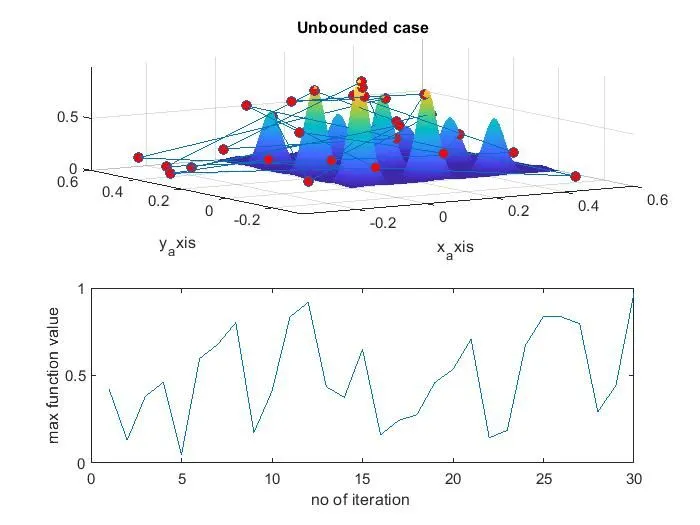
Case 1: Unbounded
case2:bounding box case
Case 3: Bounded with increased population size:
Errors faced:
Forgetting to use subplot
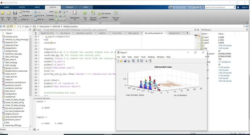
Solution: The use of subplot to get the two plots separated
Conclusion: Trough this work it is clear that stalagmite function is powerful and useful to solve complex optimization problems.
References:
https://www.sciencedirect.com/topics/engineering/genetic-algorithm
https://in.mathworks.com/help/gads/what-is-the-genetic-algorithm.html