Week 5 - Curve fitting

WEEK – 3

CURVE FITTING USING PYTHON

OBJECTIVE :

• To find the meaning of popt and pcov .
• To find the error between the curve fit data and the original data .
• To write the code for the same .

Now here is the below code for the same with proper explaination .

import math
import matplotlib.pyplot as plt
import numpy as np
from scipy.optimize import curve_fit

# Now first we will open the file and start to read it

inputfile = open('data', 'r')

# We are defining the function to read the data line by line and to mention the name of the specified coloumn . 

def readfile() :
    temp = [] 
    cpdata = []

     # It will read throughout the data one by one 

    for i in inputfile : 

        values = i.split(',')
        temp.append(float(values[0]))
        
       
        cpdata.append(float(values[1]))

    return [temp ,cpdata]

# Now defining the first function which the curfit has to take place which is a quadratic function .

def func(t,a,b,c) : 
    return a*pow(t,2) + b*t + c 

temp,cpdata = readfile() 
# Now here to remove the confusion , i have mentioned popt and pcov as x and y in simple language where x dentoes the the constant values.

x , y = curve_fit(func,temp,cpdata) 
predicted_cp_1 = func(np.array(temp) , *x)

# plot the given values .

plt.figure(1)
plt.plot(temp,cpdata, color = "blue" , linewidth = 3)
plt.plot(temp,predicted_cp_1 ,color = "red" , linewidth = 3)
plt.legend(['actual data', 'curve fit'])
plt.xlabel('temp')
plt.ylabel('cp')
plt.show()

# Now defining the first function which the curfit has to take place which is cubic function .

def func1(t,a,b,c,d) : 
    return a*pow(t,3) + b*pow(t,2) + c*t + d 



x1 ,y1 = curve_fit(func1,temp,cpdata) 
predicted_cp_2 = func1(np.array(temp) ,*x1)

# plot the values

plt.figure(2)
plt.plot(temp,cpdata, color = "yellow" , linewidth = 3)
plt.plot(temp,predicted_cp_2 ,color = "pink" , linewidth = 3)
plt.legend(['actual data', 'curve fit'])
plt.xlabel('temp')
plt.ylabel('cp')
plt.show()

# Now defining the first function which the curfit has to take place which is a bi-quadratic function .

def func2(t,a,b,c,d ,e) : 
    return a*pow(t,4) + b*pow(t,3) + c*pow(t,2) + d*t + e  


x2 ,y2 = curve_fit(func2,temp,cpdata) 
predicted_cp_3 = func2(np.array(temp) ,*x2)

# plot the values 

plt.figure(3)
plt.plot(temp,cpdata, color = "yellow" , linewidth = 3)
plt.plot(temp,predicted_cp_3 ,color = "pink" , linewidth = 3)
plt.legend(['actual data', 'curve fit'])
plt.xlabel('temp')
plt.ylabel('cp')
plt.show()


# Now after evaluation of these 3 curves , we have to find which curve is best curvefit . 
#For this we have the formulas of the errors as given in matlab course .

''' 
Now some usefull fullforms 

SSE = sum of squared errors
SSR = sum of squared regressions 
RSME = (sse/n)*0.5
SST = ssr +sse
R_SQUARE = ssr/sst

'''

s = np.sum(cpdata)
n = len(cpdata) 

mean = s/n 

# for quadratic fit

quadratic_SSR = 0
quadratic_SSE = 0

for i in range(n) :

    quadratic_error = abs(np.sum(cpdata[i]) - predicted_cp_1[i])
    quadratic_SSR =  quadratic_SSR + np.sum(pow(predicted_cp_1[i] - mean , 2))
    quadratic_SSE =  quadratic_SSE + pow(quadratic_error,2)


SSR_1 = quadratic_SSR
SSE_1 = quadratic_SSE
SST_1 = SSR_1 + SSE_1 
RSQUARE_1 = SSR_1/SST_1
RSME_1 = pow((SSE_1/n ),0.5)

print('the value of RSQUARE_1 is : ' , RSQUARE_1)
print('the value of RSME_1 is : ' , RSME_1)
print('the value of SST_1 is : ' , SST_1)

# for cubic fit

cubic_SSR = 0
cubic_SSE = 0

for j in range(n) :

    cubic_error = abs(np.sum(cpdata[j]) - predicted_cp_2[j])
    cubic_SSR =  cubic_SSR + np.sum(pow(predicted_cp_1[j] - mean , 3))
    cubic_SSE =  cubic_SSE + pow(cubic_error,2)


SSR_2 = cubic_SSR
SSE_2 = cubic_SSE
SST_2 = SSR_2 + SSE_2 
RSQUARE_2 = SSR_2/SST_2
RSME_2 = pow((SSE_2/n ),0.5)

print('the value of RSQUARE_2 is : ' , RSQUARE_2)
print('the value of RSME_2 is : ' , RSME_2)
print('the value of SST_2 is : ' , SST_2)

# for bi - quadratic  fit

bi_quadratic_SSR = 0
bi_quadratic_SSE = 0

for k in range(n) :

    bi_quadratic_error = abs(np.sum(cpdata[k]) - predicted_cp_3[k])
    bi_quadratic_SSR =  bi_quadratic_SSR + np.sum(pow(predicted_cp_1[k] - mean , 4))
    bi_quadratic_SSE =  bi_quadratic_SSE + pow(bi_quadratic_error,2)


SSR_3 = bi_quadratic_SSR
SSE_3 = bi_quadratic_SSE
SST_3 = SSR_3 + SSE_3
RSQUARE_3 = SSR_3/SST_3
RSME_3 = pow((SSE_3/n ),0.5)

print('the value of RSQUARE_3 is : ' , RSQUARE_3)
print('the value of RSME_3 is : ' , RSME_3)
print('the value of SST_3 is : ' , SST_3)

Here are the plot for the same :

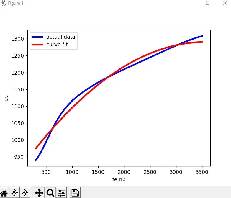
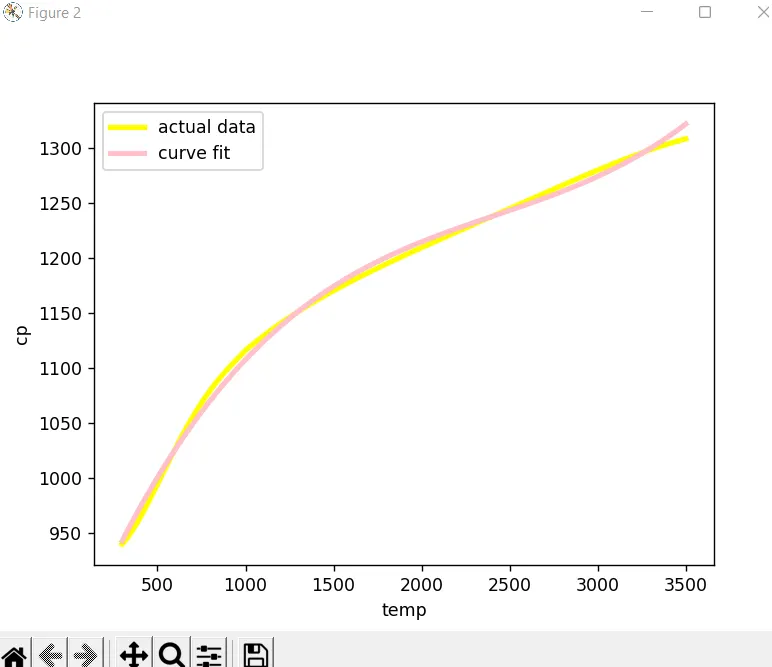
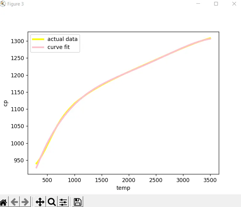
Now here is the following result for the errors :

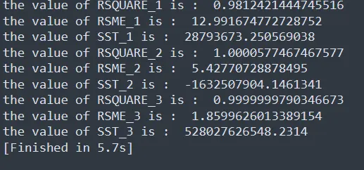
Now after analysing the result ,

we observe that the bi - quadratic function has its maximum value for Rsquare and minimum value of RSME .

So this descibes that it is the best fit .

RESULT :

1) popt ( here x) = It means it is the matrix which containes the cofficient values according the polynomial .

2) pcov ( here y ) = it means that is the matrix of the estimated values of covariance and the cofficients

3) The function of np.array(temp) does that it makes the complete of the temp values in data file by using the numpy module .

4) *popt = It stores the value of cofficients and use it to make the array of the curvefit .

5) In order to make the the fit perfect we have to increase the degree of the polynomial so that te rsquare value approches to 1 and RSME value should become minimum as possible .