Project 1 - Parsing NASA thermodynamic data
PROJECT : 1
PARSING THE NASA THERMODYNAMIC DATA
AIM :
- To extract the coefficient from the data file for the particular species and find the value of entropy , enthalpy and cp for the same .
- To plot these values for the local temperature ranges
- Also to create the code for finding the molecular weight for every compound .
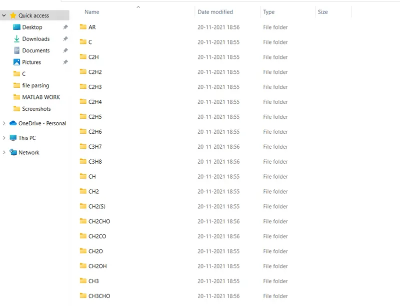
- Save the plot as images for each compound in the separate folder with the name as per preferred compound .
Code :
Read the following code line wise and you will understand the logic very clearly .
close all
clear all
clc

% opening the data file and directing it towards the matlab and assigning
% it with the variable file_id

file_id = fopen('THERMO.dat' , 'r') ;
file_line = fgetl(file_id) ;
temp = fgetl(file_id ) ; % it reads the line in data file
% the data file line is a entire string which is seperated into cells
s = strsplit(temp) ;
global_low_temp = str2double(s{2}) ; % it converts the string into numeric
global_med_temp = str2double(s{3});
global_high_temp = str2double(s{4});

% we dont want to read the next 3 lines
for i = 1 : 3
    skip =fgetl(file_id)
end

% as there are 53 different compounds ,  we have created a loop for it

for j = 1 : 53

species_header = fgetl(file_id) ; % this is the O line
local_temp_header = strsplit(species_header) ;


% Obtaining the local low temp values for a particular species

species_name = local_temp_header{1} ;

% here (end -3) is used because end is a fixed location through which we can
% change our temp values throughout the data .

local_low_temp = str2double(local_temp_header{end -3}) ;
local_med_temp = str2double(local_temp_header{end- 1}) ;
local_high_temp = str2double(local_temp_header{end -2}) ;

% extracting the string coff into numeric coff for each of the line

coeff_line1_O = fgetl(file_id) ;
coeff_line1 = strfind(coeff_line1_O,'E') ;

% determining the location of E and then determing the location of all coff in the string
a1 = str2double(coeff_line1_O(1:coeff_line1(1)+3)) ;

a2 = str2double(coeff_line1_O(coeff_line1(1)+4:coeff_line1(2)+3)) ;
a3 = str2double(coeff_line1_O(coeff_line1(2)+4:coeff_line1(3)+3)) ;
a4 = str2double(coeff_line1_O(coeff_line1(3)+4:coeff_line1(4)+3)) ;
a5 = str2double(coeff_line1_O(coeff_line1(4)+4:coeff_line1(5)+3)) ;


coeff_line2_O = fgetl(file_id) ;
coeff_line2 = strfind(coeff_line2_O,'E') ;
a6 = str2double(coeff_line2_O(1:coeff_line2(1)+3)) ;
a7 = str2double(coeff_line2_O(coeff_line2(1)+4:coeff_line1(2)+3)) ;
a8 = str2double(coeff_line2_O(coeff_line2(2)+4:coeff_line1(3)+3))  ;
a9 = str2double(coeff_line2_O(coeff_line2(3)+4:coeff_line1(4)+3))  ;
a10 =str2double(coeff_line2_O(coeff_line2(4)+4:coeff_line1(5)+3))  ;


coeff_line3_O = fgetl(file_id) ;
coeff_line3 = strfind(coeff_line3_O,'E') ;
a11 = str2double(coeff_line3_O(1:coeff_line1(1)+3)) ;
a12= str2double(coeff_line3_O(coeff_line1(1)+4:coeff_line1(2)+3)) ;
a13= str2double(coeff_line3_O(coeff_line1(2)+4:coeff_line1(3)+3))  ;
a14= str2double(coeff_line3_O(coeff_line1(3)+4:coeff_line1(4)+3))  ;

% For low temp ranges we know the coff are from the last and for high temp
% ranges we have coff from the begin  .


R  = 8.314 ;
T = linspace(local_low_temp ,local_high_temp , 100) ;
for k = 1 : length(T)
    % We have set 1500K temp as a med temp as we know the temp is
    % fluctuating

      if k>1500
          % cp = specific heat
          % H = enthalpy
          % S = entropy

cp = (a1 + a2.*T + a3.*T.^2 + a4.*T.^3 + a5.*T.^4).*R ;
H = (a1 + (a2.*T)./2 + (a3.*T.^2)/3 + (a4.*T.^3)/4 + (a5.*T.^4)/5 +a6./T).*T*R ;
S = (a1*log(T) + a2.*T +  (a3.*T.^2)/2 + (a4.*T.^3)/3 + (a5.*T.^4)/4 +a7)*R  ;

      else
cp = (a8 + a9.*T + a10.*T.^2 + a11.*T.^3 + a12.*T.^4)*R ;
H = (a8 + (a9.*T)./2 + (a10.*T.^2)/3 + (a11.*T.^3)/4 + (a12.*T.^4)/5 +a13./T).*T*R ;
S = (a8*log(T) + a9.*T +  (a10.*T.^2)/2 + (a11.*T.^3)/3 + (a12.*T.^4)/4 +a14)*R;
      end
end

% This is done to calculate the molecular weight od every compound

 w = Molecular_weight(species_name) ;
element = ['H','C','N','O','A'];
atomic_weight = [1.007,12.012,14.432,16.543,39.543];

w = 0;

for i=1:length(species_name)

  for j=1:length(element)

  if strcmp(species_name(i),element(j))


         w = w + atomic_weight(j) ;

         x = j ; % x is basically the position

  end
  end

  n = str2num(species_name(i)) ;

  if n>1

       w = w+ atomic_weight(x)*(n-1) ;
  end

end

% to display it in the command window
fprintf('molecular weight of %s :-  ' , species_name) ;
fprintf('%f', w) ;
disp(' ')
end
% Plot of  entropy , enthalpy and cp vs temp for each compound .

figure(1)

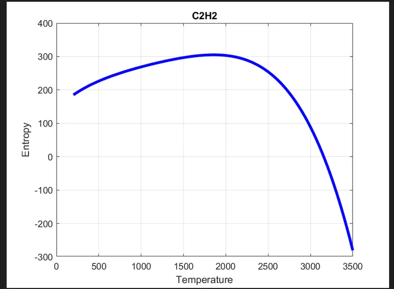
plot(T , S , 'lineWidth', 3 ,  'color' , 'b')
title(species_name)
xlabel('Temperature')
ylabel('Entropy')
grid on

figure(2)
plot(T , cp , 'lineWidth', 3 , 'color' , 'r')
title(species_name)
xlabel('Temperature')
ylabel('cp')
grid on

figure(3)
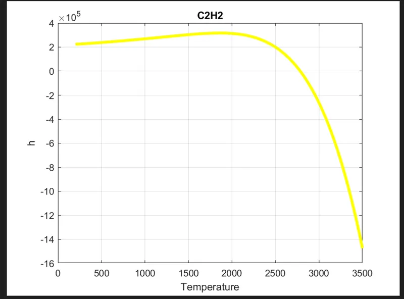
plot(T , H , 'lineWidth', 3 , 'color' , 'y')
title(species_name)
xlabel('Temperature')
ylabel('h')
grid on

% saving the each plot image inoto differnt folder of the particular
% compound mentioned

mkdir('C:\Users\Devansh\Desktop\MATLAB WORK\file parsing',species_name)
cd(species_name)
saveas(figure(1), 'entropy.png')
saveas(figure(2), 'cp.png')
saveas(figure(3), 'enthalpy.png')
cd('C:\Users\Devansh\Desktop\MATLAB WORK\file parsing')
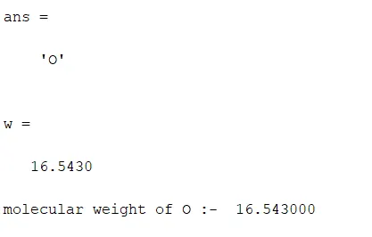
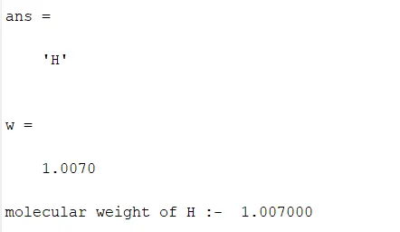
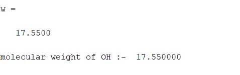
Molecular weight in command window :
Various plot :
For the compound carbon we have :
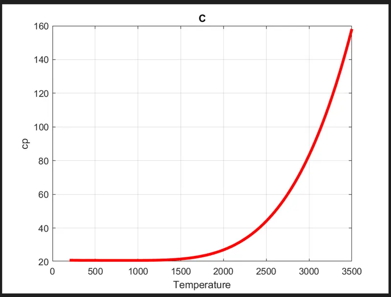
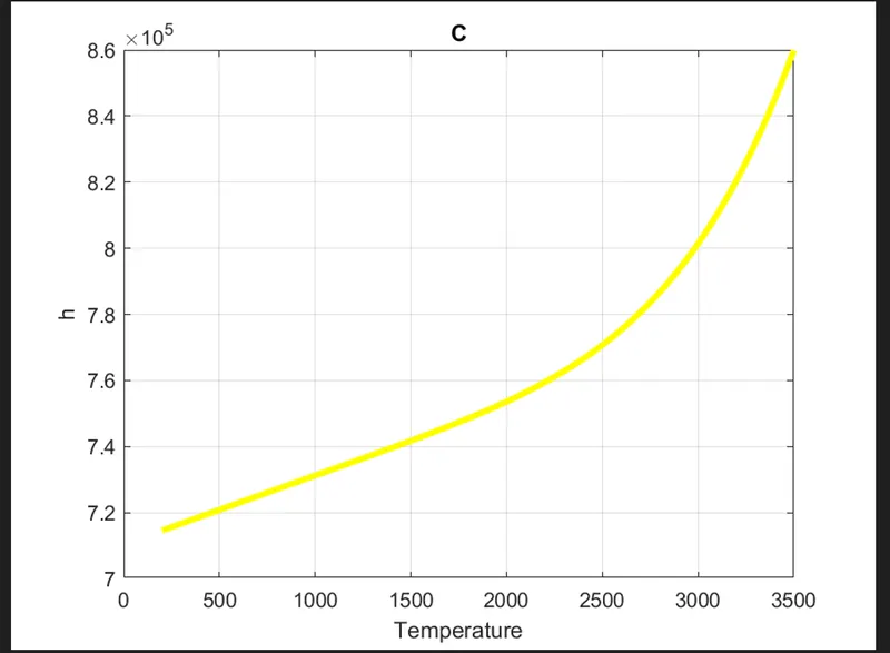
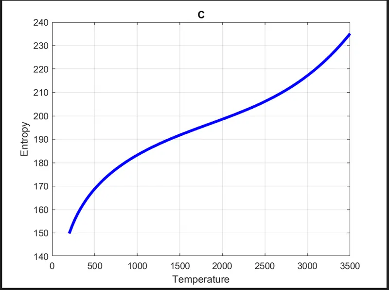
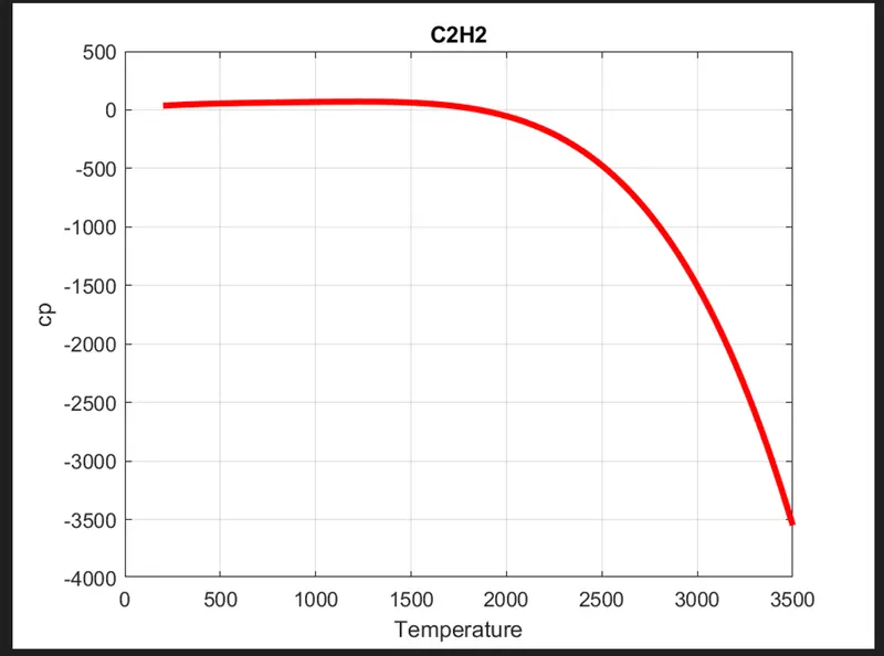
For the compound C2H2 we have :
All these plots are saved in the same directory :