Week 3 - Solving second order ODEs

WEEK – 3

AIM : Complete MATLAB program to simulate the pendulum motion for a given period .

EXPLANATION :

LINES	EXPLANATION
2 - 7	The input variables are assigned as per the equation .
9 - 10	Time period is given for the motion
12 – 14	Initial condition are given for pendulum as when t = 0 [ displacement ; velocity ] is [ 0 ; 3 ] .
17 -19	This is the ODE function equation in which the motion will be executed for different time period
23 - 28	Now for different time , the function will be executed . Now since x1 y1 are the coordinates of the pendulum , it is clear that the result vector from the ODE will be equal to the displacement vector , that is 1 column .
32	This is a line plotted for the base for the motion to be done by the line of pendulum
33	Hold on is used as to plot all the points an lines at once to avoid the plot of the last command .
34	Marker command is used for plotting the ball in the graph
44	Hold off command is used to remove the initial frame of the ball so that it does not fix for the second frame to happen .
48 - 58	Code for making the animation .
63 - 72	The output of this function is a column vector because the initial condition was also a column vector and to make the output more clear we have used various terms .

ERRORS AND STEPS TAKEN TO OVERCOME :

• The animation was not there as there was a continuous set of images by not using the hold off command .

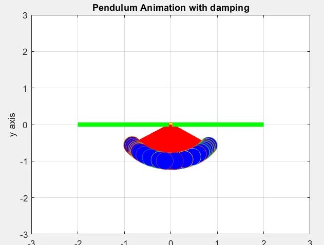
2 ) Writing color in marker instead of markerfacecolor .

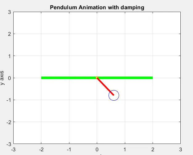
• Not incrementing the counter by 1 in the for loop .

code :

% inputs variables assigned where b is the damping coffiecient .

g = 9.81 ;
l = 1 ;
m =1 ;
b = 0.05 ;

% time for simulation
t_span = linspace(0 , 20 , 200) ;

% initial condition 

time_0 = [0 ; 3] ;


% ODE as function of time and theta 

[t , results ] = ode45(@(t , theta) ode_func(t , theta , b , g , l ,  m ) , t_span , time_0 ) 

ct =1 ;

for i = 1 : length(t_span)
    x0 = 0 ;
    y0 = 0 ;

    x1 =  -l*sin(results(i,1))
    y1 =  -l*cos(results(i,1))
      
figure (1)
    
    plot([-2 2] , [0 0] , 'linewidth' , 5 , 'Color', 'g') ;
    hold on
    plot(x0,y0 , 'o' ,'markersize' , 5 , 'markerfacecolor', 'y' )
    plot([ x0 x1] , [y0  y1] ,  'linewidth' , 3 , 'Color', 'r' )
    plot( x1 ,y1 , 'o' ,'markersize' , 20, 'markerfacecolor', 'b' )
  
    axis ([-3 3 -3 3]) ;
    grid on 
    
    xlabel( 'x axis')
    ylabel('y axis')
    title('Pendulum Animation with damping' )
    hold off
   
    pause(0.03)
    
    M(ct) = getframe(gcf) ; 
    ct = ct + 1 ;  % counter frame to be incremented by 1 to avoid mismatch of the incomplete M array .
end

% command for the animation 

movie(M) 
videofile = VideoWriter('pendulum.avi' , 'uncompressed AVI') ; 
open(videofile)
writeVideo(videofile,M)
close(videofile)

% function 

function  [output] = ode_func(t , theta, b , g , l ,  m )

 
 dtheta1_dt = theta(2) ;
 dtheta2_dt = (-b/m)*theta(2) - (g/l)*sin(theta(1)) ;


output = [dtheta1_dt ; dtheta2_dt] ; 

end 

https://www.youtube.com/watch?v=PC8abfOkzOI

Conclusion :

Able to draw the the damped pendulum animation and can see different observation by changing different value of damping cofficient .