Week 2 Air standard Cycle

WEEK-2 - AIR STANDARD CYCLES

ENGINE KINEMATICS

AIM : 1) to plot a PV diagram of otto cycle .

2) To calculate the thermal efficiency of the cycle .

Below is the given code , read it properly , you will understand the logic and code .

import math
import matplotlib.pyplot as plt
import numpy as np
import scipy 

# first of all we are defining the function for the trace of volume between any two points .
# the main reason is to calculate and call the function for different values of the crank angle in the process of expansion and compression 

def funcmain(bore, stroke, cr , cond_rod , start_crank , end_crank):
    
    # inputs assigned 

    bore  = 0.1
    stroke = 0.1
    cr = 12
    cond_rod = 0.15
    a = stroke/2
    r = cond_rod/a
    # crank angle is calculated in radians . 
    sc = math.radians(start_crank)
    ec = math.radians(end_crank)

    theta = np.linspace(sc, ec , 10)  # It is an array between the sc and ec to trace the volume in the bore at  10 different values
    swept_vol  = math.pi*(1/4)*pow(bore,2)*stroke
    v_c = swept_vol/(cr -1)

    # Now this volume trace is the equation of the trace mentioned in the for loop

    Volume_trace = []

    for i in theta :
        

	

        term_1 = (cr - 1)/2
        term_2 = r +1 - math.cos(i) 
        term_3 = pow(r,2) -pow(math.sin(i),2)
        term_3 = pow(term_3,0.5)	
        Volume_trace.append((1 + term_1*(term_2 - term_3))*v_c) # this volume trace is also an array now pf 10 values

    return(Volume_trace)



bore  = 0.1
stroke = 0.1
cr = 12
cond_rod = 0.15
a = stroke/2
r = cond_rod/a
gamma = 1.4

swept_vol  = math.pi*(1/4)*pow(bore,2)*stroke
v_c = swept_vol/(cr -1)

# state parameters at state 1 
v1 =  swept_vol  + v_c 
p1 = 101325  # given
t1 = 500   # given

# state parameters at state 2
v2 =  v_c
p2 = p1*pow(v1,gamma)/pow(v2,gamma)
x = p1*v1/t1
t2 = p2*v2/(x)

# Now we will find the actual path between these 2 points  by calling the function 

constant  = p1*pow(v1,gamma)  # by formula 

Compression_volume_trace = funcmain(bore, stroke, cr , cond_rod , 180, 0)

Compression_pressure_trace = []

for i in Compression_volume_trace :
    Compression_pressure_trace.append(constant/(pow(i,gamma)))

# state parameters at state 3
v3 = v2
y = p2*v2/t2
t3 =2300  # given 
p3 = y*t3/v3

# Now we will join these state 2 and 3 points as volume is same 

Constant  = p3*pow(v3,gamma)

expansion_volume_trace = funcmain(bore, stroke, cr , cond_rod , 0, 180)

expansion_pressure_trace = []

for i in expansion_volume_trace :
    expansion_pressure_trace.append(Constant/(pow(i,gamma)))


# state parameters at state 4

v4 = v1
p4 = p3*pow(v3,gamma)/(pow(v4,gamma))
t4 = p4*v4*t3/(p3*v3)

# Now we will find the actual path between these 2 points  by calling the function .

# after this we will finally plot all the points and the path between these . 

plt.plot(v1,p1,marker='*')
plt.plot(Compression_volume_trace , Compression_pressure_trace) 
plt.plot(v2,p2,marker='*') 
plt.plot(v3 , p3 , marker='*')
plt.plot([v2,v3] , [p2,p3])
plt.plot(expansion_volume_trace , expansion_pressure_trace)
plt.plot(v4 ,p4 ,marker='*' )
plt.plot([v4,v1], [p4,p1])
plt.xlabel("volume")
plt.ylabel("pressure")
plt.show()

# efficincy of the cycle :

eta = (1-(1/(pow(cr,0.4))))*100
print('thermal eff of cycle is ',eta,'%')

Below is the plot given

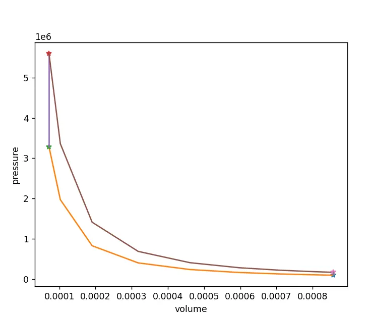
Also eff :

eta = 62.9%