Week 5 - Curve fitting

Curve fitting:-

Curve fitting is the process of constructing a curve, or mathematical function, that has the best fit to a series of data points, possibly subject to constraints. Curve fitting can involve either interpolation, where an exact fit to the data is required, or smoothin, in which a "smooth" function is constructed that approximately fits the data. A related topic is regression analysis,which focuses more on questions of statistical inference such as how much uncertainty is present in a curve that is fit to data observed with random errors. Fitted curves can be used as an aid for data visualization, to infer values of a function where no data are available,and to summarize the relationships among two or more variables. Extrapolation refers to the use of a fitted curve beyond the range of the observed data,and is subject to a degree uncertainty since it may reflect the method used to construct the curve as much as it reflects the observed data.

popt : array

Optimal values for the parameters so that the sum of the squared error of {f(xdata, *popt) - ydata} is minimized

pcov : 2d array

The estimated covariance of popt. The diagonals provide the variance of the parameter estimate. To compute one standard deviation errors on the parameters use{ perr = np.sqrt(np.diag(pcov))}.

popt,pcov=curve_fit(func_linear,temperature,cp)

np.array(temperature):-This function stores the temperature values in the form of array and passes it to the function numpy.

in *popt:- It stores the values of the parameter of the function.

coding for curve fitting

objectives

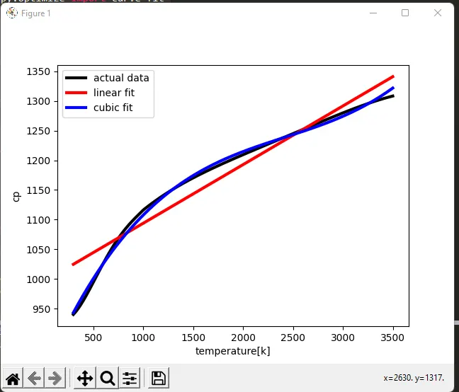
2. make the plot with curve fits and actual data

code:-

import numpy as np
import matplotlib.pyplot as plt
from scipy.optimize import curve_fit

#curve fit function 
#linear fit function
def func_linear(t,a,b):
	return a*t+b
#cubic fit function
def func_cubic(x,a,b,c,d):
	return a*pow(x,3)+b*pow(x,2)+c*x+d

#reading the thermodynamic data file 
def read_file():
	temperature=[]
	cp=[]
	for line in open('data','r'):
		values=line.split(',')
		temperature.append(float(values[0]))
		cp.append(float(values[1]))
	return[temperature,cp]

#main program
temperature,cp=read_file()
popt,pcov=curve_fit(func_linear,temperature,cp)
popx,pcov=curve_fit(func_cubic,temperature,cp)

fit_cp1=func_linear(np.array(temperature),*popt)
fit_cp2=func_cubic(np.array(temperature),*popx)
#to check the best fit 
sse=0
for i in range(0,np.size(cp)):
	sse1=sse+pow(cp[i]-fit_cp1[i],2)
	sse2=sse+pow(cp[i]-fit_cp2[i],2)
 

#R_square
mean=np.sum(cp)/np.size(cp)
ssr=0
for i in range(0,np.size(cp)):
	ssr1=ssr+pow(fit_cp1[i]-mean,2)
	ssr2=ssr+pow(fit_cp2[i]-mean,2)

sst1=ssr1+sse1
R_square1=ssr1/sst1
sst2=ssr2+sse2
R_square2=ssr2/sst2

print("R_square for linear fit =",R_square1)
print("R_square for cubic fit =",R_square2)
#ploting
plt.plot(temperature,cp,color="black",linewidth=3)
plt.plot(temperature,fit_cp1,color="red",linewidth=3)
plt.plot(temperature,fit_cp2,color="blue",linewidth=3)
plt.legend(['actual data','linear fit','cubic fit'])
plt.xlabel('temperature[k]')
plt.ylabel('cp')
plt.show()

code explanation:-

1. Initially Importing the required modules
2. defining the function for linear fit and cubic fit
3. Reading the thermodynamic data file by defining function read_file()
4. spliting values at ',' and float the values
5. main programing starts by calling the function read_file()
6. fiting cp linear and cubic
7. To check the best fit by using formulas (sse=sum of square of errore) and (ssr=sum of square of regersion)
8. making of plots ,legend, labels

output:-

conclusion:-

In order to make perfect fit, we must consider error estimates as well. Perfect fit means, the curve should fit the original curve without showing any errors (such as centering and scaling erros) in that perticular degree of polynomial. Perfect fit can always be a best fit but best fit can not be a perfect fit.In this case cubic fit is perfect

The ranges to define our results

1. If R_square=1,then our results is perfect
2. If R_square=0.95-0.99,then the results is good
3. If R_square<=0.94,the results are bad

our results

R_square for linear fit = 0.9591952791481255
R_square for cubic fit = 0.9907133759605077
both fits are not perferct but cubic fit is good from both.