Week 3 - Solving second order ODEs

AIM : To generate a plot for a Simple Pendulum and create the animation for the same.

INTRODUCTION :

A simple pendulum is an arrangement in which a weighted mass is suspended with the help of a string, which is fixed at one end and free at another end.This weighted mass free to move in space when provide with an external force.When the mass is displaced sideways from its equilibrium postion it is subjected to restoring force due to gravity,which tries to pull it back to equilibrium posistion.This restoring force tends to ossicillates the mass about its equilibrium position moving it back and forth.This motion of the pendulum will keep going until the restoring force is less than the gravity and the frictional force due to the surrounding atmosphere.

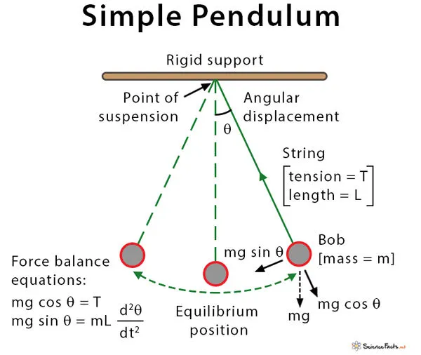
The motion of the pendulum is a circular arc.Every motion of the pendulum will make an angle with the vertical axis.This angle defines the amplitude of the oscillatory motion in the vertical plane,greater the angle higher are the oscillations and bigger ids the arrc created by the bob.We have to solve the angle to trace the motion path of the bob,to find the change in velocity according to the time.

GOVERNING EQUATION :

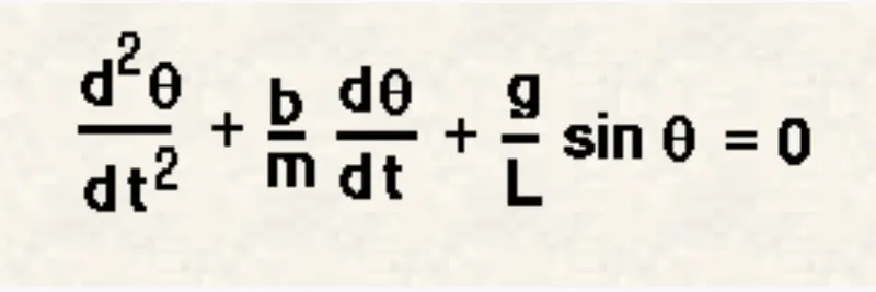
In the above equation that represents the motion of the pendulum in air is

Where,

b=Dampinng Force,

m=Mass of the bob,

g=acceleration due to gravity (9.81m/s) and

l=length of the string.

This is a second order differential equation,which first needs to be simplifed for the angle and can be directly solve in the Matlab for the time and velocity plot of the motion.Later this output can be used for generating the animation of the moving pendulum.

To solve this equation we need to convert it into a first-order ODE.Which then can be used as an input function in the code,and by using the ode45 command we can compute the results by givivng proper initial conditions and input parameters.

MATLAB CODE :

function [dtheta_dt]=ode_func(t,theta,b,g,l,m)
theta1=theta(1)
theta2=theta(2)
dtheta1_dt=theta2;
dtheta2_dt=-(b/m)*theta2-(g/l)*sin(theta1);
dtheta_dt=[dtheta1_dt;dtheta2_dt];
end

EXPLANATION :

• In the above code,we have created a function that represents the given IDE for simple pendulum.
• The input for the function is time,theta,b,g,l,m using the inputs we can solve the ODE and generate the output.
• We have simplifed the second order ODE into first order ODE and included two variables for them theta1 and theta2.This two variables that will be defining our output vector of the ODE.
• In this function,wwe have included the angles,the simplied form of our second-order ODE,and the solution matrix.

clear all
close all
clc


b = 0.05;
g = 9.81;
l = 1;
m = 1;

%Initial condition
theta_0=[0;3];

%Time points
t_span = linspace(0,10,500);

%Solve ODE
[t,results] = ode45(@(t,theta)ode_func(t,theta,b,g,l,m),t_span,theta_0);
hold on
plot(t,results(:,1))
hold on
plot(t,results(:,2))
xlabel('time')
ylabel('amplitude')
grid on

legend({'Displacement(rad)','Velocity(rad/sec)'})
ct=1;

for i=1:length(t_span)
    theta = results(:,1)
    
    x0=0;
    y0=0;
    x1=-l*sin(theta(i));
    y1=-l*cos(theta(i));
    
    %plotting
    figure(2)
    plot([-1 1],[0 0],'linewidth',35,'color','black');
    hold on
    plot([x0 x1],[y0 y1],'linewidth',1.75);
    hold on
    plot(x1,y1,'.','markersize',75)
    hold off
    grid on
    %limits of axis
    axis([-1 1 -1 1]);
    pause(0.1)
    %collecting frames of figures to create animation
    M(ct)=getframe(gcf);
    ct=ct+1;
end

movie(M)
videofile=VideoWriter('simple_pendulem.avi','uncompressed AVI');
open(videofile)
writeVideo(videofile,M)
close(videofile)

EXPLANATION :

1. First,we entered our inputs variables that are b,m,l,g and ct .Along with that,we had our initial conditions for displacement and velocity i.e.,0 meters and 3rad/sec respectively.
2. Next,we introduced the time vector,as we have to simulate the motion between 0-20 seconds we will be using the linspace command to generate the time vector.
3. With the using the command ode45 we will introduce the ode solver into our code.(t,theta) are the variables defining the ode,second_orderODE_pendulum(t,theta,b,g,l,m) is the function that we created,t_span is the time vector that will change according to time,theta_0 are initial conditions for the function.
4. This solver will be solving the ode as per the inputs and initial conditions that are provided.
5. The next step will be plotting the velocity and displacement profile.The x and y axis will havetime and velocity respectively.By using simple plotting command we can easily plot the output of the ode that is solved.
6. Now to generate the animation of the plot,first we will a variable theta2 to the results that are generated.Then this variable will be introduced into a for loop which will later be assigned the steps to a new variable theta_x.
7. By giving the conditions for the string i.e.,x0 and y0 is the fixed point of the string and the other point will be difened by x1 and y1 which will change w.r.t time.
8. For plotting the animation first we will be plotting the fixpoint of the animation,next will be the string that is attached t the fixed point and the bob at the other end,at the last we will be using the marker command to plot the bob.
9. For generating the movie first we will be creating an array 'M' which will be storing the frames generated,ct is the counter that will be incrementing the frame count.
10. VideoWriter will help us to generate the avi file for the animation.First,we will be opening the video file,writeVideo will write the videofile and using array M,finally we will be closing the videofile.

OUTPUT :

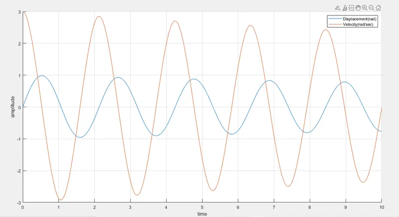
• This is the velocity,time and displacement plot generated by the above code.Red is velocity as the nitial conditions show velocity is 3rad/sec intially and blue is the displacement as it starts from 0 meters.

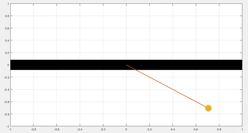
• The geometry that was plotted using the commands will be animated.

LINK FOR THE ANIMATION AND OUTPUY FILE :

https://youtu.be/_rXcu40n0dU

ERRORS :

1. theta0 must be entered as theta_0 since in function program it is called like that.

2. The input ct was not given by assigning the value the error corrected.

CONCLUSION :

• The above work can be conclude that Matlab can be used for solving the ode of any order of any order mentioned.As seen in the output plot the displacement of the pendulum was slowly getting reduced because of the damping provided.The amplitude vs the velocity is also decreasing as the time passes by.
• The animation generated is also supporting the results that we concluded,as the time proceeds the bob slow down and the amplitude of the swing reduces.