Week 3 - Solving second order ODEs

AIM : To generate a plot for a Simple Pendulum and create the animation for the same.

INTRODUCTION :

A simple pendulum is an arrangement in which a weighted mass is suspended with the help of a string, which is fixed at one end and free at another end.This weighted mass free to move in space when provide with an external force.When the mass is displaced sideways from its equilibrium postion it is subjected to restoring force due to gravity,which tries to pull it back to equilibrium posistion.This restoring force tends to ossicillates the mass about its equilibrium position moving it back and forth.This motion of the pendulum will keep going until the restoring force is less than the gravity and the frictional force due to the surrounding atmosphere.

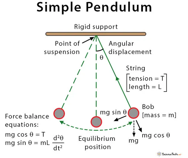
The motion of the pendulum is a circular arc.Every motion of the pendulum will make an angle with the vertical axis.This angle defines the amplitude of the oscillatory motion in the vertical plane,greater the angle higher are the oscillations and bigger ids the arrc created by the bob.We have to solve the angle to trace the motion path of the bob,to find the change in velocity according to the time.

GOVERNING EQUATION :

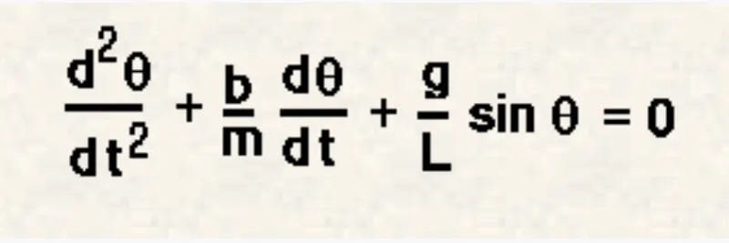
In the above equation that represents the motion of the pendulum in air is

Where,

b=Dampinng Force,

m=Mass of the bob,

g=acceleration due to gravity (9.81m/s) and

l=length of the string.

This is a second order differential equation,which first needs to be simplifed for the angle and can be directly solve in the Matlab for the time and velocity plot of the motion.Later this output can be used for generating the animation of the moving pendulum.

To solve this equation we need to convert it into a first-order ODE.Which then can be used as an input function in the code,and by using the ode45 command we can compute the results by givivng proper initial conditions and input parameters.

Python code :

import math
import numpy as n1
import matplotlib.pyplot as plt
from scipy.integrate import odeint

def model(initial,t,b,l,g,m):
	t1=initial[0]
	t2=initial[1]
	dt1=t2
	dt2=(-b*t2/m)-(g*math.sin(t1)/1)
	dt=[dt1,dt2]
	return dt

b=0.05
l=1
g=9.81
m=1

initial=[0,3]
t=n1.linspace(0,20,200)
disvelo=odeint(model,initial,t,args=(b,l,g,m))

plt.plot(t,disvelo[:,0],'-',label='displacement')
plt.plot(t,disvelo[:,1],'--',label='velocity')
plt.legend()
plt.xlabel('time')
plt.ylabel('displacementvelocity')
plt.show()

y=disvelo[:,0]
ct=1
for ang in y:
	x1=0;y1=0
	x2=l*math.sin(ang)
	y2=-l*math.cos(ang)
	file='test%05d.png'%ct
	plt.figure()
	plt.plot([-1.5,1.5],[0,0],linewidth=8)
	plt.plot([x1,x2],[y1,y2],linewidth=3)
	plt.plot(x2,y2,'o',markersize=15)
	plt.xlim([-1.5,1.5])
	plt.ylim([-1.5,1.5])
	plt.savefig(file)
	ct=ct+1