Week 5 - Curve fitting

Q1. What does popt and pcov mean?

Ans.

'popt' represents the matrix which stores and extracts the coefficients for the fitting functions according to the general equations defined.

popt : array, Optimal values for the parameters so that the sum of the squared residuals of f(xdata, *popt) - ydata is minimized

'pcov' represents the square matrix which stores the estimated values of covariance of the coefficients of the above. The diagonal element of this square matrix also represents variance of that coefficients.

pcov : 2d array

The estimated covariance of popt. The diagonals provide the variance of the parameter estimate. To compute one standard deviation errors on the parameters, use perr = np.sqrt(np.diag(pcov)). How the sigma parameter affects the estimated covariance depends on absolute_sigma argument, as if True, sigma is used in an absolute sense and the estimated parameter covariance pcov reflects these absolute values. If False, only the relative magnitudes of the sigma values matter. The returned parameter covariance matrix pcov is based on scaling sigma by a constant factor.

Q2. What does np.array(temperature) do?

Ans. Using the numpy module, this programme turns each temperature value in the data file into an array.

Q3. What does the * in *popt mean?

Ans. '*', '*popt' indicates and returns each coefficient stored in popt array.

Q4. What needs to be done in order to make the curve fit perfect?

Ans. When the order of the polynomial is increased, the inaccuracy created decreases and the curve fits properly. When the rank of the polynomial is increased, the value of 'R2' approaches 1 and is deemed to be a perfect match.

This approach is time-consuming since it necessitates defining functions for each new polynomial. Instead of using this approach, one of the data sets, such as temperature, may be divided into many domains. For example, if the temperature column has 5000 values, we can divide it into 10 domains of 500 values, which will fit nicely on a curve if plotted.

Procedure:

1. The first line in this programme will be a comment statement, after which we will begin importing libraries such as math, scipy, matplotlib, and numpy.
2. Then we'll define the polynomial function, which will include all of the variables and constants.
3. We'll now read the data file and import the temperature and cp value from it.
4. Now we'll begin curve fitting, reading the thermodynamic data file first and then determining the arbitrary constant value of the polynomial equation.
5. Finally, we'll plot the raw data as well as the curve fit data line.
6. We'll use this method to fit third-order polynomials.
7. After plotting curve fit goodness is calculated.

Code:

#importing modules and libraries
import numpy as np 
import matplotlib.pyplot as plt 
from scipy.optimize import curve_fit

# Curve_fit function for linear polynomial 
def func(t, a, b):
	return a*t + b

# Curve_fit function for cubical polynomial 
def func_1(t, a, b, c, d):
	return a*pow (t,3) + b*pow(t,2) + c*t +d 

# Reading thermodynamic data file 
def read_file ():
	temp = []
	cp = []
	for line in open('data', 'r'):
		values = line.split(',')
		temp.append(float(values[0]))
		cp.append(float(values[1]))

	return [temp, cp]

#Main programs
temp, cp = read_file()

#linear
popt, pcov = curve_fit(func, temp, cp)
fit_cp_1 = func(np.array(temp), *popt)

#linear curve fit plotting
plt.figure(1)
plt.plot(temp, cp, 'k--')
plt.plot(temp, fit_cp_1,, linewidth= 1)
plt.legend(['Actaual_data', 'Curve_fit'])
plt.xlabel('Temperature [k]')
plt.ylabel('c_p')
plt.title('Linear Curve Fitting')
plt.show()

print('\n')

#cubic
popt, pcov = curve_fit(func_1, temp, cp)
fit_cp_2 = func_1(np.array(temp), *popt)

#cubic curve fit plotting
plt.figure(2)
plt.plot(temp, cp,'k--')
plt.plot(temp, fit_cp_2,, linewidth = 1)
plt.legend(['Actaual_data', 'Curve_fit'])
plt.xlabel('Temperature [k]')
plt.ylabel('c_p')
plt.title('cubical Curve Fitting')
plt.show()

''' 
Measuring the fitness characetristics of the curves
SSE = (sum of error squared)
SSR = (sum of square of the regression)
SST = SSE + SSR
R^2 = SSR/SST
RMSE = (SSE/1)^0.5

finding mean of cp data
mean = (sum of all elements)/(total number of elements)
'''
s = np.sum(cp)
l = np.size(cp)
m = s/l 
print ('\nMean of all cp :', m)
print('')

# For a linear curve fit

linear_sse = 0
linear_ssr = 0
for i in range(1):
	linear_error = abs((np.sum((cp[i] - fit_cp_1[i]))))
	linear_sse = linear_sse+pow(linear_error,2)
	linear_ssr = linear_ssr+ np.sum(pow((fit_cp_1[i] - m),2))

linear_sst = linear_sse + linear_ssr
print('linear_sst :', linear_sst)
linear_R2 = linear_ssr/linear_sst
print('linear_R2 :', linear_R2)
linear_rmse = pow((linear_sse/1),0.5)
print('linear_rmse :', linear_rmse)
print('')

# For cubic curve fit

cubic_sse = 0
cubic_ssr = 0
for j in range(1):
	cubic_error = abs((np.sum((cp[j] - fit_cp_2[j]))))
	cubic_sse = cubic_sse+pow(cubic_error,2)
	cubic_ssr = cubic_ssr+ np.sum(pow((fit_cp_2[j] - m),2))

cubic_sst = cubic_sse + cubic_ssr
print('cubic_sst :', cubic_sst)
cubic_R2 = cubic_ssr/cubic_sst
print('cubic_R2 :', cubic_R2)
cubic_rmse = pow((cubic_sse/1),0.5)
print('cubic_rmse :', cubic_rmse)
print('')

Output:

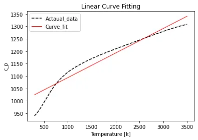
Linear curve fit:

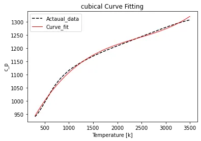
Cubic curve fit:

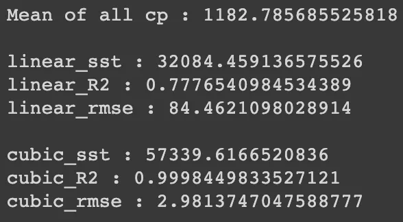
Curve fit goodness:

Conclusion:

As a result, it indicates that the bend fit great R2 should be close to 1. It is clear from the results that R2 for straight bend fit is approximately 0.93, and R2 for cubic bend fit is around 0.99. As a result, it's common to say that cubic polynomials fit better than straight polynomials. The estimation of R2 will crawl towards 1 as the request for the polynomial grows, and fit will be considered satisfactory.