Week 5 - Curve fitting

Ans. 1) popt is the array that stores all the values of the polynomial coefficients computed from the input data. pcov is the resultant covariance matrix that indicates how these coefficients change together.

Ans. 2) np.array(temperature) arranges the values of temperature in an equally spaced manner in an array.

Ans. 3) the * in *popt helps refer to the correct elements of the popt array when the array is being used in a function. This allows to pass the array itself as a argument for the said function, rather than its individual elements.

Skill-lync project 2

Aim: The objective of this assignment is to create a Python code that can fit a linear and a cubic curve to the set of provided data points.

Problem statement: The curve fitting code is required for specific heat data from a text document. The document contains 2 sets of data; one corresponding to temperature and the other corresponding to specific heat. The curve is to depict the relation between these two parameters. The relation is to be depicted via a linear and a cubic curve.

Theory: Curve fitting is a common operation performed in statistical analyses. It is used to express the relation between two measured quantities as a polynomial equation. The purpose of this equation is to predict the value of one value with that of the other. Fitting a curve representing an n^th degree polynomial requires at least n+1 data points. The n+1 coefficients of the polynomial are then computed such that there is minimal difference between the predicted value for one data point and the actual data point.

Python’s scipy module contains the curve_fit() command that can compute all the coefficients of an n^th degree polynomial for a given set of values. These coefficients can then be used to plot the polynomial curve that can then be compared with the input data. How well the curve fits can be assessed empirically by means of the root mean squared error between the polynomial and the data. This error is given by the following formula.

Error = (1/n) * Σ(y_p-y)^2

n = Number of data points

y_p = Value of polynomial at given point

y = Value of actual data at same point

Procedure: The code for fitting the two curves is created through the following sequence of steps.

1. The first few lines of code are used to import the math, matplotlib, numpy and scipy modules.
2. The data from the text document is then extracted and their values are assigned to 2 arrays with the function shown below.

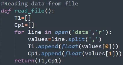
Figure 1: Function for reading data and assignment to arrays

3. Two functions line1() and cube1() are defined for the linear and cubic curves that are to be fitted to the data, as shown below.

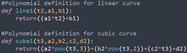
Figure 2: Functions for linear and cubic curves

4. The curve_fit() command is then used to fit both the curves to the data.
5. The output of the curve_fit consists of an array of the computed coefficient values assigned to the variables topt1 & topt2 for each of the 2 curves, and a square covariance matrix assigned to the variables tcov1 & tcov2, as shown below.

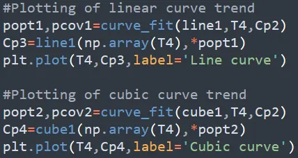
Figure 3: Unpacking of curve_fit() output and plotting of polynomial curves

The covariance matrix gives a measure of how the coefficients of the polynomial change together.

6. The two curves are then plotted on the same figure, along with the original data, in order to show the accuracy of these curves.
7. Finally, the root mean squared error for both the curves are printed using the following lines of code, and compared.

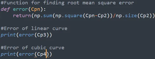
Figure 4: Function for computing root mean square error

Result: The final code for the curve fitting algorithm is shown below.

#Imported modules
import math
import matplotlib.pyplot as plt
import numpy as np
from scipy.optimize import curve_fit

#Reading data from file
def read_file():
	T1=[]
	Cp1=[]
	for line in open('data','r'):
		values=line.split(',')
		T1.append(float(values[0]))
		Cp1.append(float(values[1]))
	return(T1,Cp1)

#Polynomial definition for linear curve
def line1(t2,a1,b1):
	return((a1*t2)+b1)

#Polynomial definition for cubic curve
def cube1(t3,a2,b2,c2,d2):
	return((a2*pow(t3,3))+(b2*pow(t3,2))+(c2*t3)+d2)

#Plotting of input data
T4,Cp2=read_file()
plt.plot(T4,Cp2,label='Actual data')

#Plotting of linear curve trend
popt1,pcov1=curve_fit(line1,T4,Cp2)
Cp3=line1(np.array(T4),*popt1)
plt.plot(T4,Cp3,label='Line curve')

#Plotting of cubic curve trend
popt2,pcov2=curve_fit(cube1,T4,Cp2)
Cp4=cube1(np.array(T4),*popt2)
plt.plot(T4,Cp4,label='Cubic curve')

#Display of plots
plt.xlabel('Temperature (K)')
plt.ylabel('Specific heat (J/kg*K)')
plt.legend()
plt.savefig('Final curve fit')

#Function for finding root mean square error
def error(Cpn):
	return(np.sum(np.square(Cpn-Cp2))/np.size(Cp2))

#Error of linear curve
print(error(Cp3))

#Error of cubic curve
print(error(Cp4))

The temperature vs. specific heat plot for the original data and the two polynomial curves are shown below.

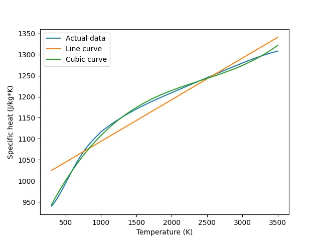Figure 5: Final plot of data and polynomial curves

It shows that of the two polynomial curves, the cubic curve provides the better fit to the given input data. However, even this cubical curve is not perfect, as at the tail end of that curve, it begins to deviate from the input data.

Ultimately, this graph shows that there are two approaches to making the best fitting curve for a given data set. The first approach is to use a polynomial with the highest possible degree. The second approach is to use a piecewise linear polynomial. In this case the turning point for this polynomial can exist at the temperature of 1000 K.

The root mean square error for the linear curve is computed to be 675.95, while that for the cubic curve is computed to be 29.46. The lower error value of the cubic curve confirms the observation that it is a better fit for the data than the linear curve.

Conclusions: The curve fitting algorithm has been successfully implemented and the suitability of higher order polynomials for this purpose has been successfully demonstrated.