Week 5 - Curve fitting

Curve fitting

1. AIM:

Write a codes to perform curve fitting in Python.

2. OBJECTIVES:

- Develop code to fit a linear and cubic polynomial for the Cp data.
- Graph the linear and cubic fit curves along with the raw data points.
- Evaluate the fitness characteristics for both the curves.

3. GOVERNING EQUATIONS:

Data spread could be represented using curve fitting, which assigns the best fit function along with the entire range.
The are diferent types of curve fitting like:
Interpolation, a function exact fit to the data points and has limited applicability to real-life scenarios.
Smoothing, a function that fit the data points aproximately and the error is minimized overall.

Linear curve fitting refers to a straight line that fits adequately to the data. The equation of a generic straight line is always given by f(x)= a x + b.
Polynomial curve fitting refers to a polynomial function.

There are four parameters that allow to measure how well the equations are representing the given data points:
- The sum of squares dueto error (SSE),
- R-square (R2),
- Adjusted R-square,
- Root mean squared error (RMSE)

4. CONTENT OF THE BODY:

The python code that was created is shown below.

# Linear and cubic polynomial curve fitting
# By Pablo Jimenez

import math
import matplotlib.pyplot as plt
import numpy as np
from scipy.optimize import curve_fit

# Curve fit function

# Linear function
def function_1(t,a,b):
	return a*t + b

# Cubic function
def function_2(t,a,b,c,d):
	return a*pow(t,3) + b*pow(t,2) + c*t +d

# Reading thermodynamic data file
def read_file():
	temp = []
	cp = []
	for line in open('data','r'):
		values = line.split(',')
		temp.append(float(values[0]))
		cp.append(float(values[1]))
	return [temp , cp]

# Main Program
temp,cp = read_file()
popt,pcov = curve_fit(function_1,temp,cp)
fit_cp_l = function_1(np.array(temp),*popt)
plt.figure(1)
plt.plot(temp,cp,'b--',linewidth = 1)
plt.plot(temp,fit_cp_l,color='black',linewidth = 1)
plt.legend(['Actual data','Curve fit'])
plt.xlabel('temp (K)')
plt.ylabel('Cp')
plt.title('Linear curve fitting')
plt.show()

popt,pcov = curve_fit(function_2,temp,cp)
fit_cp_c = function_2(np.array(temp),*popt)
plt.figure(3)
plt.plot(temp, cp,'b--',linewidth = 1)
plt.plot(temp, fit_cp_c,color='black',linewidth = 1)
plt.legend(['Actual data','Curve fit'])
plt.xlabel('temp (K)')
plt.ylabel('Cp')
plt.title('Cubic Curve fitting')
plt.show()

# Measuring the fitness characetristics of the curves
# SSE (sum of error squared)
# SSR (sum of squares of the regression)
# SST = SSE + SSR
# R^2 = SSR/SST
# RMSE = (SSE/1)^0.5

s = np.sum(cp)
l = np.size(cp)
m= s/l
print('Mean of all cp :',m)
print('')

# For Linear curve fit
linear_sse = 0
linear_ssr = 0
for i in range(1):
	linear_error = abs((np.sum((cp[i] - fit_cp_l[i]))))
	linear_sse = linear_sse+pow(linear_error,2)
	linear_ssr = linear_ssr+ np.sum(pow((fit_cp_l[i] - m),2))

linear_sst = linear_sse + linear_ssr
print('Linear_sst :',linear_sst)
linear_R2 = linear_ssr/linear_sst
print('Linear_R2 :',linear_R2)
linear_rmse = pow((linear_sse/l),0.5)
print('Linear_RMSE :',linear_rmse)
print('')

# For Cubic curve fit
cubic_sse = 0
cubic_ssr = 0
for j in range(1):
	cubic_error = abs(np.sum((cp[i] - fit_cp_c[i])))
	cubic_sse = cubic_sse+(pow(cubic_error,2))
	cubic_ssr = cubic_ssr+np.sum(pow((fit_cp_c[i]-m),2))

cubic_sst = cubic_sse + cubic_ssr
print('Cubic_sst :',cubic_sst)
cubic_R2= cubic_ssr/cubic_sst
print('Cubic_R2 :',cubic_R2)
cubic_rmse = pow((cubic_sse/l),0.5)
print('Cubic_RMSE :',cubic_rmse)

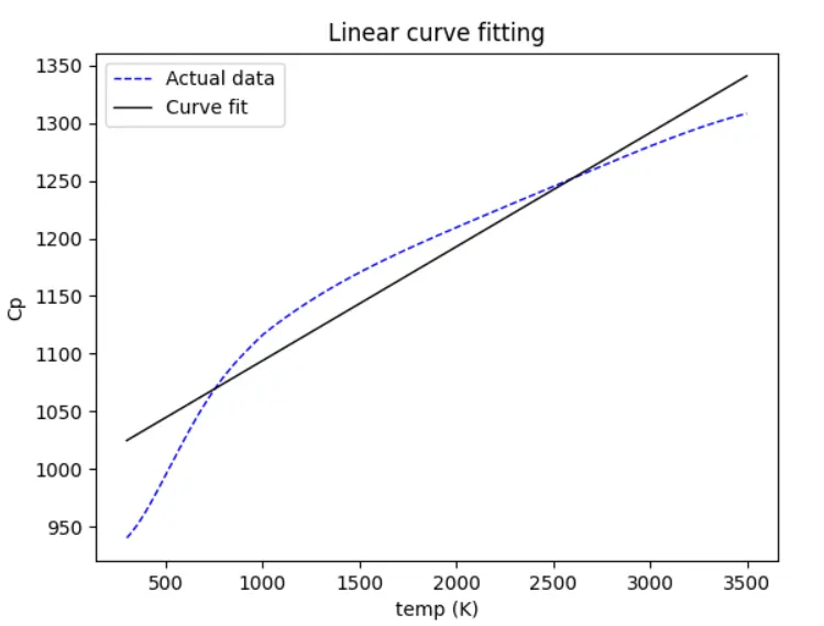
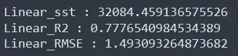
The graph of the linear curve is represented in the next figure.

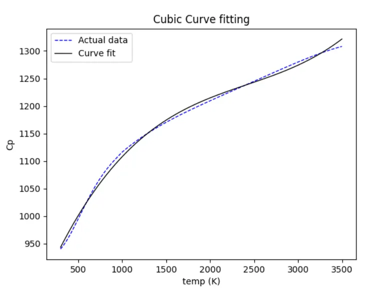
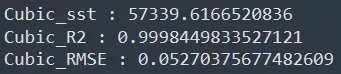
For the cubic curve fitting, the graph obtained is the next one.

Based on the analysis presented above, the following questions are answered:
Q1. What does popt and pcov mean?
A. 'popt' is the matrix which stores and extracts the coefficients for the fitting functions according to the general equations defined.
‘pcov' represents the square matrix which stores the estimated values of covariance of the coefficients of the above. The diagonal element of this square matrix also represents variance of that coefficients.

Q2. What does np.array(temperature) do?
A. This command converts each data of temperature in the file into an array using numpy module.

Q3. What does the * in *popt mean?
A. "*", "*popt" indicates and returns each coefficients stored in popt array.

Q4. What needs to be done in order to make the curve fit perfect?
A. If we increase the order of the polynomial, the error produced will be less and curve fit perfectly.

5. CONCLUSION:

- The straight line has a R^2 is around 0.93 and for cubic bend fit it is about 0.99. So it tends to be said that cubic polynomial fits superior to straight regression.