Week 3 - Solving second order ODEs

Solving second order ODEs

1. AIM:

- Simulate the the motion of a damped pendulum in Python.

2. OBJECTIVE:

- Write a program that solves the equation of motion of a simple pendulum with damping.

- Create a simulation of the motion of the pendulum.

3. GOVERNING EQUATION:

A simple pendulum is composed of a mass (m) hanging from a string of length (l) and negligible mass, fixed at a pivot point P. When the mass is displaced an initial angle and is released, the pendulum will swing back and forth with periodic motion around an equilibrium position located at the lowest point of the trajectory, it is shown in the following figure.

In more realistic situations, inevitably the pendulum is losing energy due to frictional forces and, in consequence, its amplitude decreases with time. In this way, a non-conservative force which is proportional to the pendulum speed is assumed. This force can be written as:

`F_f = -b*v`

Where b is a positive constant which depends on the medium, materials, and also on the body shape.

Finally, the ODE is defined as:

`(d^2theta)/dt^2+b/m*(d theta)/dt+g/l*sin(theta)=0`

4. BODY OF THE CONTENT:

The code in Python to solve the ODE and graph the pictures for the animation is shown below.

import numpy as np
import math
from scipy.integrate import odeint
import matplotlib.pyplot as plt

# Funcontion
def model(T,t,b, L, g,m):
	T1 = T[0]
	T2 = T[1]
	dT1_dt = T2
	dT2_dt = -(b/m)*T2 -(g/L)*math.sin(T1)
	dTh_dt = [dT1_dt, dT2_dt]
	return dTh_dt

# Inputs
b = 0.05 # damping co-efficient
L = 1 # L of pendulum in m
g = 9.81 # g in m/s%*2
m = 1 # m of ball in kg
# initial conditions
T_x = [0,3]
# time points
t = np.linspace(0,20,200)
# solve ode
T = odeint(model,T_x,t,args=(b,L,g,m))

# Plot
plt.plot(t,T[:,0],'b-',label = r'$\frac{d\theta_1}{dt}=\theta_2$' )
plt.plot(t,T[:,1],'g--',label= r'$\frac{d\theta_2}{dt}=-\frac{b}{m}\theta_2-\frac{g}{l}sin\theta_1$')
plt.ylabel('Displacement / Velocity')
plt.xlabel('Time')
plt.legend(loc='best')
plt.grid()
plt.show()

# Figures for animation
X = T[:,0]
cont =1
for theta in X:
	x1 = 0
	y1 = 0
	x2 = L*math.sin(theta)
	y2 = -(L*math.cos(theta))
	file = 'test%05d.png'%cont
	plt.figure()
	plt.plot([x1,x2],[y1,y2],linewidth = 2,color='k')
	plt.plot(x2,y2,'o',markersize =21,color='r')
	plt.xlim([-1.5,1.5])
	plt.ylim([-1.5,1.5])
	plt.savefig(file)
	cont = cont+1

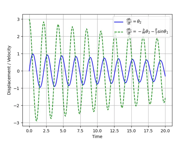
The graph of the displacement and the angular velocity is shown.

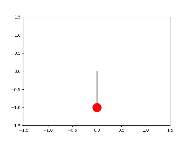
And the simulation is exemplified.

Link: https://youtu.be/RU4HtfaTjrM

5. CONCLUSIONS:

- The behavior of a damped pendulum was estimated. The graph showed the angular displacement and angular velocity and it changes over the time due to the effect of the damping.

- The simulation of the movement of the pendulum was completed.