Week 2 Air standard Cycle

Air standard Cycle

1. AIM:

- Write a program to solve an Otto cycle and perform plots for it in Python.

2. GOVERNING EQUATIONS:

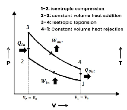
The Otto cycle is refered to the thermodynamic cycle related to spark-ignition reciprocating engines. In this way, an Otto ideal cycle completes four processes: Two isentropic and two isochoric.

`C_v`

Process 1-2: Isentropic Compression

In this process, the movement of the piston is from Top Dead Center (TDC) to Bottom Dead Center (BDC).

- Pressure increases from P1 to P2.

- Volume decreases from V1 to V2.

- Temperature rises from T1 to T2.

- Entropy remains constant.

Process 2-3: Constant Volume Heat Addition

The piston rest for a moment at TDC and during this process,

- Pressure increases from P2 to P3.

- Volume remains constant (V2=V3).

- Temperature increases from T2 to T3.

- Entropy increases from S2 to S3.

In this process:

`Heat supplied = m*C_v*(T_3-T_2)`

Where

m is the mass of the fluid

`C_v` is the specific heat at a constant volume

Process 3-4: Isentropic Expansion

The piston moves from TDC to BDC.

- Pressure decreases from P3 to P4.

- Volume increases from V3 to V4.

- Temperature falls from T3 to T4.

- Entropy remains unchanged.

Process 4-1: Constant Volume Heat Rejection

The piston rest for a moment a BDC and rejection of heat take place at constant volume.

- Pressure decreases from P4 to P1.

- Volume remains constant (V4=V1)

- Temperature falls from T4 to T1.

The value of heat rejected in this process is calculated as:

`Heat rejected = m*C_v*(T_4-T_1)`

Where

m is the mass of the fluid

`C_v` is the specific heat at a constant volume

Thermal efficiency of an ideal Otto Cycle

`eta_(th)=1-(T_4-T_1)/(T_3-T_2)`

Where

`eta_(th) is the thermal efficiency`

3. OBJECTIVES OF THE PROJECT:

- Solve the Otto cycle and plot its p-V diagram.

- Calculate the thermal efficiency of the mentioned Otto cycle.

4. BODY OF THE CONTENT:

The code implemented in Python is shown below.

"""
Program of an Otto ideal cycle
By Pablo Jimenez
"""
import math
import matplotlib.pyplot as plt

# Inputs
gamma = 1.4
T3 = 2300 # max temp inside engine cylinder
p1 = 101325
T1 = 350

# Engine geometry properties
bore = 0.15
stroke = 0.2
conn_rod = 0.8
c_r = 10

# Calculating swept volume and clearance volume
v_s = (math.pi/4)*pow(bore,2)*stroke
v_c = v_s/(c_r -1)
v1 = v_s + v_c
v2 = v_c

def engine_kinematics(bore, stroke, conn_rod,c_r,start_crank_angle,end_crank_angle):
	
	# Engine geometry properties
	r = stroke/2
	n = conn_rod/r
	
	# Volume parameters
	v_s = (math.pi/4)*pow(bore,2)*stroke
	v_c = v_s/(c_r -1)

	theta_startcrank = math.radians(start_crank_angle)
	theta_endcrank = math.radians(end_crank_angle)
	
	n_val = 100
	dtheta = (theta_endcrank - theta_startcrank)/(n_val - 1)
	V=[]
	for i in range(0,n_val):
		theta = theta_startcrank + i*dtheta
		term_1 = 0.5*(c_r - 1)
		term_2 = n + 1 - math.cos(theta)
		term_3 = (pow(n,2) - pow(math.sin(theta),2))
		term_3 = pow(term_3,0.5)
		V.append((1 + term_1*(term_2 -term_3))*v_c)
	return V

# Process 2
# p2*v2%gamma = p1*vi*gamma
p2 = p1* pow(c_r,gamma)
# (p1*v1)/T1 = (p2*v2)/T2 | T2 = p2*v2*T1/(p1*v1)
T2 = p2*v2*T1/(p1*v1)
V_comp = engine_kinematics(bore, stroke, conn_rod,c_r,180,0)
C_const = p1*pow(v1, gamma)
P_comp = []
for v in V_comp:
	P_comp.append(C_const/pow(v,gamma))

# Process 3
v3 = v2 # Isochoric process
# (p3*v3)/T3 = (p2*v2)/T2 | p3 = p2*T3/(T2)
p3 = p2*T3/(T2)
V_expp = engine_kinematics(bore, stroke, conn_rod,c_r,0,180)
C_const = p3*pow(v3,gamma)
P_expp = []
for v in V_expp:
	P_expp.append(C_const/pow(v,gamma))

# Process 4
v4 = v1 # Isochoric process
# p3*v3^gamma = p4*v4^gamma # Isentropic expansion process
p4 = p3*pow(v3,gamma)/pow(v4,gamma)
# (p3*v3)/T3 = (p4*v4)/T4 | T4 = p4*v4*T3/(p3*v3)
T4 = p4*v4*T3/(p3*v3)

#p-V Graph
plt.plot(V_comp,P_comp)
plt.plot([v2,v3],[p2,p3])
plt.plot(V_expp,P_expp)
plt.plot([v4,v1],[p4,p1])
plt.ylim([-500000,8000000])
plt.xlim([0,0.005])
plt.xlabel('Volume (m^3)')
plt.ylabel('Pressure(Pa) ')
plt.title('p-V diagram of an Otto Cycle')
plt.grid()
plt.show()

#Thermal efficiency
thermal_efficiency = 1-((T4-T1)/(T3-T2))
print('Thermal efficiency of given Otto Cycle is :',thermal_efficiency)

The following plot for the p-V curve was observed, after running the code.

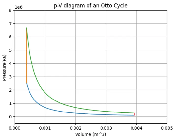
Additionally, the thermal efficiency of the cycle was calculated.

5. CONCLUSIONS:

Using Python,P-V diagram is plotted and the thermal efficiency of the cycle was estimated.