Week 5 - Curve fitting

AIM:

Understand the basic concepts of Curve Fitting using Python and answer the given questions.

THEORY:

Curve Fitting : It is the process of constructing a curve or a mathematical function, that has a best fit to a series of data points, possibly subject to constraints. Curve fit can involve either interpolation, where an exact fit to the data is required, or smoothing, in which a "smooth" function is constructed that approximately fits the data. A related topic is regressional analysis, which focuses more on questions of more statistical inference such as how much uncertainty is present in the curve that is fit to data observed with random errors. Fitted curves can be used as an aid for data visualization, to infer values of a function where no data are available, and to summarize the relationships among two or more variables. Extrapolation refers to the use of a fitted curve beyond the range of the observed data, and subject to a degree of uncertainty since it may reflect the method used to construct the curve as much as it reflects the observed data.

CODE:

# For Linear Function
import matplotlib.pyplot as plt
from scipy.optimize import curve_fit
import numpy as np
# Curve Fit Polynomial Function
def func(x,a,b,c):
	return a*x+b
# File parsing
def read_file():
	temperature=[]
	Cp=[]
	for line in open('data1','r'):
		values=line.split(",")
		temperature.append(float(values[0]))
		Cp.append(float(values[1]))
	return [temperature, Cp]
temperature, Cp=read_file()
popt, pcov=curve_fit(func, temperature, Cp)
fit_cp=func(np.array(temperature), *popt)
# Graph Plotting
plt.plot(temperature,Cp,linewidth=3)
plt.plot(temperature,fit_cp,linewidth=3)
plt.legend(['Actual Data','Curve Fit'])
plt.xlabel('Temperature [K]')
plt.ylabel('Cp')
plt.grid()
plt.show()

# For quadratic Function

import matplotlib.pyplot as plt
from scipy.optimize import curve_fit
import numpy as np
# Curve Fit Polynomial Function
def func(x,a,b,c):
	return a*x**2+b*x+c
# File parsing
def read_file():
	temperature=[]
	Cp=[]
	for line in open('data1','r'):
		values=line.split(",")
		temperature.append(float(values[0]))
		Cp.append(float(values[1]))
	return [temperature, Cp]
temperature, Cp=read_file()
popt, pcov=curve_fit(func, temperature, Cp)
fit_cp=func(np.array(temperature), *popt)
# Graph Plotting
plt.plot(temperature,Cp,linewidth=3)
plt.plot(temperature,fit_cp,linewidth=3)
plt.legend(['Actual Data','Curve Fit'])
plt.xlabel('Temperature [K]')
plt.ylabel('Cp')
plt.grid()
plt.show()

# For Cubic Function

import matplotlib.pyplot as plt
from scipy.optimize import curve_fit
import numpy as np
# Curve Fit Polynomial Function
def func(x,a,b,c,d):
	return a*x**3+b*x**2-c*x+d
# File parsing
def read_file():
	temperature=[]
	Cp=[]
	for line in open('data1','r'):
		values=line.split(",")
		temperature.append(float(values[0]))
		Cp.append(float(values[1]))
	return [temperature, Cp]
temperature, Cp=read_file()
popt, pcov=curve_fit(func, temperature, Cp)
fit_cp=func(np.array(temperature), *popt)
# Graph Plotting
plt.plot(temperature,Cp,linewidth=3)
plt.plot(temperature,fit_cp,linewidth=3)
plt.legend(['Actual Data','Curve Fit'])
plt.xlabel('Temperature [K]')
plt.ylabel('Cp')
plt.grid()
plt.show()

RESULTS:

Here the results for the above code is as shown below -
For Linear Function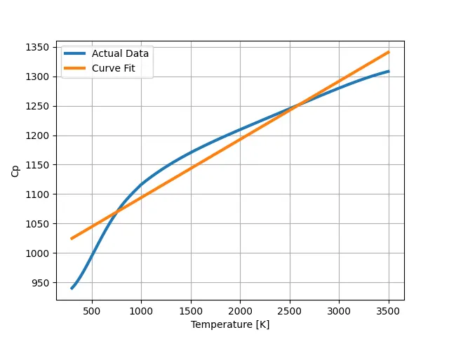

For Quadratic Function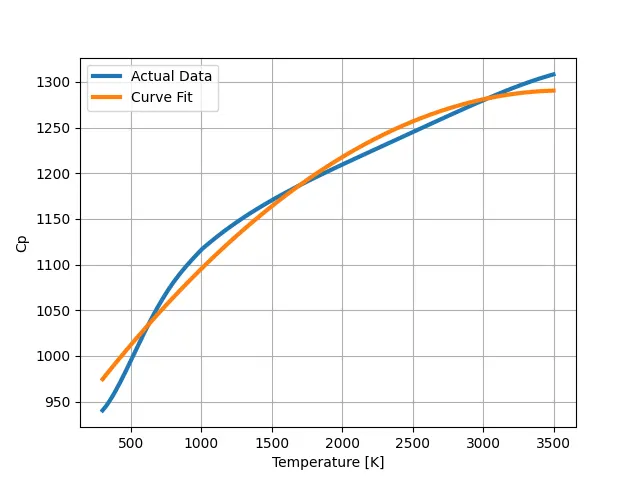

For Cubic Function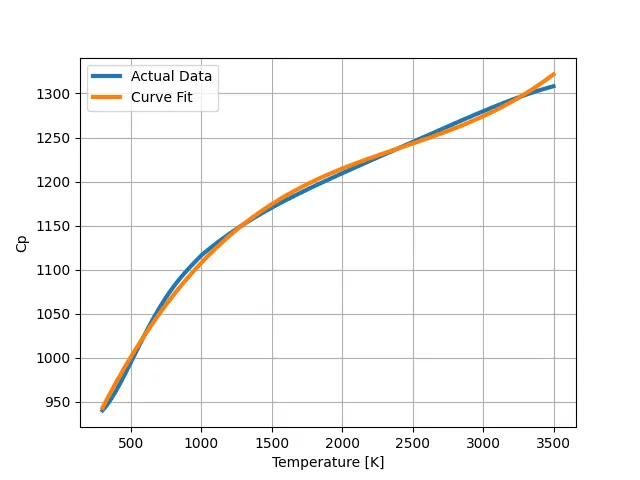

It is quite evident from the above plots that, in order to get the best fit, we need to have a higher order polynomial function. For higher order polynomial the fitted curve tends to resemble more to the actual curve. Hence higher our order of the polynomial function, better is the fit of our curve.

np.array(temperature) from our code, collects all the temperature values in an array format and is then used to provide these temperature values as the input.

Also, the pcov in our code is nothing but, 2-D array which consists of the estimated covariance of popt.

*popt in our program indicates that all the values of the popt are to be considered.