Week 5 - Curve fitting
ANSWERS
1. What does popt and pcov mean?
Ans:
popt array
popt or p optimal parameter refers to the best fit parameters for the constants.
Optimal values for the parameters so that the sum of the squared residuals of f(xdata, *popt) - ydata is minimized.
pcov 2-D array
pcov contains the covariance matrix which indicates the uncertainities and correlations between the parameters. or it is the estimated covariance of popt. The diagonals provide the variance of the parameter estimate. To compute one standard deviation errors on the parameters use perr = np.sqrt(np.diag(pcov)).
2.What does np.array(temperature) do?
Ans:
Numpy arrays are great alternatives to Python Lists. Some of the key advantages of Numpy arrays are that they are fast, easy to work with, and give users the opportunity to perform calculations across entire arrays.
The program below shows how np.array function works:
import numpy as np
rawdata=[1,2,3,4,5]
print("RAWDATA")
print(rawdata)
print("rawdata when called using np.array function:")
arr = np.array(rawdata)
print(arr)
print("rawdata when called as such:")
print(rawdata)
The outpit looks like:
RAWDATA
[1, 2, 3, 4, 5]
rawdata when called using np.array function:
[1 2 3 4 5]
rawdata when called as such:
[1, 2, 3, 4, 5]
Similarly the function np.array(temperature) will only take the numerical values of temperature
3. What does the * in *popt mean?
Ans: popt parameters are the best fit parameters (p optimal) for the constants like a,b,c etc in the function defined.So here *popt will refer to the whole set of the constants a.b.c etc.It simply gives the array of a,b,c etc.Please refer the code below to get an idea regarding the same.
#CASE 2- FITTING A HIGHER ORDER POLYNOMIAL MODEL
def func(x,a,b,c,d,e):
    return a*pow(x,4)+b*pow(x,3)+c*pow(x,2)+d*x+e
popt,pcov=curve_fit(func,temperature,cp)
print("HIGHER ORDER POLYNOMIAL FITTING")
print('\n')
print("The optimum values of a,b,c,d and e are: ")
print(popt)
output will give:
HIGHER ORDER POLYNOMIAL FITTING


The optimum values of a,b,c,d and e are:
[-1.02120102e-11  9.66516802e-08 -3.36791972e-04  5.82718379e-01
  7.81066722e+02]
Here as the constants are a,b,c,d and e ,we get the 5 popt values.So when *popt is said,it refers to the 5 values of a,b,c,d and e.
4. Write code to fit a linear and cubic polynomial for the Cp data. Explain if your results are good or bad.
Ans.A program with full explanation for performing curve fitting in python is attached below.We have performed the curve fitting for 4 function and the best fit one is determined.
#PROGRAM FOR FITTING A CURVE BETWEEN TEMPERATURE AND Cp VALUES GIVEN
#CREATED BY LAKSHMI RAJAN P
#CREATED ON 28TH MAY 2021 USING IDE NAMED SPYDER

#IMPORTING THE REQUIRED MODULES
import numpy as np
import matplotlib.pyplot as plt
from scipy import integrate
from scipy.optimize import curve_fit
import csv

#IMPORT DATA-data between temperature and cp has been provided,saved it as an csv file
#openend the file 'data.csv' in read option represented as 'r' in i
with open("data.csv",'r') as i:
    #data saved as a comma separated file is read and the values are stored as a list in rawdata
    rawdata=list(csv.reader(i,delimiter=','))
    #numpy array function calls all columns from first column and all rows and convert
    #the string values to float and store it in exampledata
exampledata=np.array(rawdata[0:],dtype=np.float)
#making the first column to give temperature values
temperature=exampledata[:,0]
#making second column as cp values
cp=exampledata[:,1]
#plotting the given data
plt.figure(1,dpi=120)
plt.plot(temperature,cp,label="experimental data")
plt.xlabel("temperature")
plt.ylabel("specific heat")

#Now we have to define a function which will suit the given data with proper fit
#CASE 1-FITTING A LINEAR MODEL
def func(x,a,b):
    return a*x+b
popt,pcov=curve_fit(func,temperature,cp)
print("LINEAR POLYNOMIAL FITTING")
print('\n')
print("The optimum values of a and b are: ")
print(popt)
print('\n')
funcdata=func(temperature,*popt)
plt.plot(temperature,funcdata,label="linear model data",color='g')
plt.legend()

#CASE 2- FITTING A QUADRATIC MODEL
def func(x,a,b,c):
   return a*pow(x,2)+b*x+c
popt,pcov=curve_fit(func,temperature,cp)
print("QUADRATIC POLYNOMIAL FITTING")
print('\n')
print("The optimum values of a,b and c are: ")
print(popt)
print('\n')
funcdata=func(temperature,*popt)
plt.plot(temperature,funcdata,label="quadratic model data",color='y')
plt.legend()

#CASE 2- FITTING A CUBIC POLYNOMIAL MODEL
#A cubic function is defined
def func(x,a,b,c,d):
    return a*pow(x,3)+b*pow(x,2)+c*x+d
#A curve is fit with the function and the data
popt,pcov=curve_fit(func,temperature,cp)
print("CUBIC POLYNOMIAL FITTING")
print('\n')
print("The optimum values of a,b,c and d are: ")
print(popt)
print('\n')

#defined a variable 'funcdata' to store the values after running the cubic function defined
#with x values taken from temperature and *popt refers to the best fit parameters for the constants
funcdata=func(temperature,*popt)
#plotting the curve defined
plt.plot(temperature,funcdata,label="cubic model data",color='b')
plt.legend()

#CASE 2- FITTING A HIGHER ORDER POLYNOMIAL MODEL
def func(x,a,b,c,d,e):
    return a*pow(x,4)+b*pow(x,3)+c*pow(x,2)+d*x+e
popt,pcov=curve_fit(func,temperature,cp)
print("HIGHER ORDER POLYNOMIAL FITTING")
print('\n')
print("The optimum values of a,b,c,d and e are: ")
print(popt)
print('\n')
funcdata=func(temperature,*popt)
plt.plot(temperature,funcdata,label="higher order model data",color='r')
plt.title("FITTING A CURVE BETWEEN TEMPERATURE AND SPECIFIC HEAT")
plt.legend()
print("The best fit is provided by the higher order polynomial as it covers the experimental data correctly")
Here we got a plot between temperature and cp for different functions.The plot is attached below:
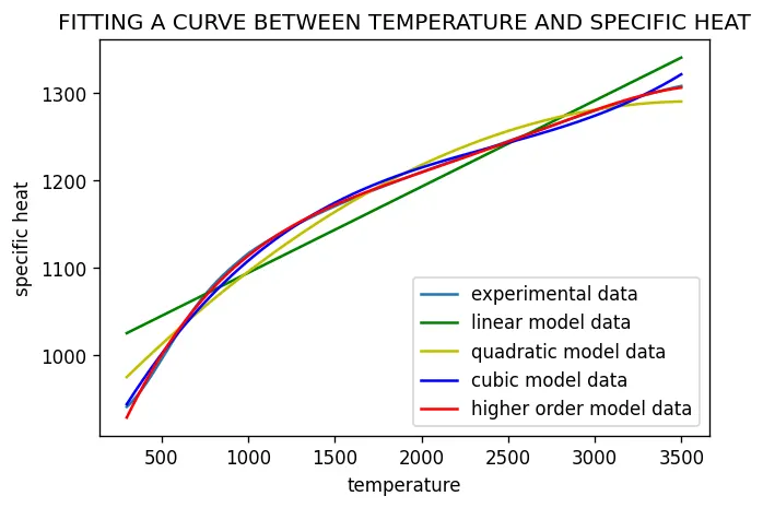
Figure 1: combined model showing the best fit curve
we can see that the higher order polynomial correctly fits the experimental data and that is the best curve fitted.
The graphs for linear and cubic polynomial is attached herewith.
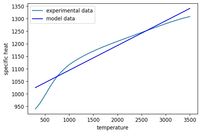
figure 2: linear model data fitted curve
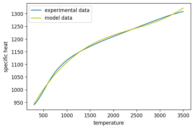
Figure 3: Cubic function fitted model with the experimental data
Comparatively between linear and Cubic model,the better fit is provided by cubic function as it covers the experimental data correctly.
5. What needs to be done in order to make the curve fit perfect?
Ans:
Curve fitting is an optimization problem that finds a line that best fits a collection of observations.
It is easiest to think about curve fitting in two dimensions, such as a graph.
Consider that we have collected examples of data from the problem domain with inputs and outputs.
The x-axis is the independent variable or the input to the function. The y-axis is the dependent variable or the output of the function. We don’t know the form of the function that maps examples of inputs to outputs, but we suspect that we can approximate the function with a standard function form.
Curve fitting involves first defining the functional form of the mapping function (also called the basis function or objective function), then searching for the parameters to the function that result in the minimum error.
Error is calculated by using the observations from the domain and passing the inputs to our candidate mapping function and calculating the output, then comparing the calculated output to the observed output.
Once fit, we can use the mapping function to interpolate or extrapolate new points in the domain. It is common to run a sequence of input values through the mapping function to calculate a sequence of outputs, then create a line plot of the result to show how output varies with input and how well the line fits the observed points.
The key to curve fitting is the form of the mapping function.
A straight line between inputs and outputs can be defined as follows:
- y = a * x + b
Where y is the calculated output, x is the input, and a and b are parameters of the mapping function found using an optimization algorithm.
This is called a linear equation because it is a weighted sum of the inputs.
In a linear regression model, these parameters are referred to as coefficients; in a neural network, they are referred to as weights.
This equation can be generalized to any number of inputs, meaning that the notion of curve fitting is not limited to two-dimensions (one input and one output), but could have many input variables.
For example, a line mapping function for two input variables may look as follows:
- y = a1 * x1 + a2 * x2 + b
The equation does not have to be a straight line.
We can add curves in the mapping function by adding exponents. For example, we can add a squared version of the input weighted by another parameter:
- y = a * x + b * x^2 + c
This is called polynomial regression, and the squared term means it is a second-degree polynomial.
So far, linear equations of this type can be fit by minimizing least squares and can be calculated analytically. This means we can find the optimal values of the parameters using a little linear algebra.
We might also want to add other mathematical functions to the equation, such as sine, cosine, and more. Each term is weighted with a parameter and added to the whole to give the output; for example:
- y = a * sin(b * x) + c
Adding arbitrary mathematical functions to our mapping function generally means we cannot calculate the parameters analytically, and instead, we will need to use an iterative optimization algorithm.
This is called nonlinear least squares, as the objective function is no longer convex (it’s nonlinear) and not as easy to solve.
So Inorder to fit the curve perfectly,we have find the function best suited for it to fit the curve.So we have to start expoloring from the linear function to further higher order polynomials and find the best fit.But going to higher,coefficients related to higher order will almost become zero and thus doe not make any sense to fit in that order.So we take up a comparatively better fitted cubic polynomial function and then split the data values to different sets.And then evaluate the function separately.
pcov gives the estimated covariance of popt.The diagonals provide the variance of the parameter estimate. To compute one standard deviation errors on the parameters use perr = np.sqrt(np.diag(pcov)).
6. Show empirically as to how well your curve has been fit.
Ans. The curve fitting has been done in two ways
1)Using the polynomial functions from linear to higher order polynomials
2)Selecting a cubic polynomial and then splitting the data and by plotting the curve
Case 1: PROGRAM CODE WITH DETAILED EXPLANATION
#IMPORTING THE REQUIRED MODULES
import numpy as np
import matplotlib.pyplot as plt
from scipy import integrate
from scipy.optimize import curve_fit
import csv

#IMPORT DATA-data between temperature and cp has been provided,saved it as an csv file
#openend the file 'data.csv' in read option represented as 'r' in i
with open("data.csv",'r') as i:
    #data saved as a comma separated file is read and the values are stored as a list in rawdata
    rawdata=list(csv.reader(i,delimiter=','))
    #numpy array function calls all columns from first column and all rows and convert
    #the string values to float and store it in exampledata
exampledata=np.array(rawdata[0:],dtype=np.float)
#making the first column to give temperature values
temperature=exampledata[:,0]
#making second column as cp values
cp=exampledata[:,1]
#plotting the given data
plt.figure(1,dpi=120)
plt.plot(temperature,cp,label="experimental data")
plt.xlabel("temperature")
plt.ylabel("specific heat")

#Now we have to define a function which will suit the given data with proper fit
#CASE 1-FITTING A LINEAR MODEL
def func(x,a,b):
    return a*x+b
popt,pcov=curve_fit(func,temperature,cp)
perr=np.sqrt(np.diag(pcov))

print("LINEAR POLYNOMIAL FITTING")
print('\n')
print("The optimum values of a and b are: ")
print(popt)
print('\n')
funcdata=func(temperature,*popt)
plt.plot(temperature,funcdata,label="linear model data",color='g')
plt.legend()

#CASE 2- FITTING A QUADRATIC MODEL
def func(x,a,b,c):
   return a*pow(x,2)+b*x+c
popt,pcov=curve_fit(func,temperature,cp)
print("QUADRATIC POLYNOMIAL FITTING")
print('\n')
print("The optimum values of a,b and c are: ")
print(popt)
print('\n')
funcdata=func(temperature,*popt)
plt.plot(temperature,funcdata,label="quadratic model data",color='y')
plt.legend()

#CASE 3- FITTING A CUBIC POLYNOMIAL MODEL
#A cubic function is defined
def func(x,a,b,c,d):
    return a*pow(x,3)+b*pow(x,2)+c*x+d
#A curve is fit with the function and the data
popt,pcov=curve_fit(func,temperature,cp)
print("CUBIC POLYNOMIAL FITTING")
print('\n')
print("The optimum values of a,b,c and d are: ")
print(popt)
print('\n')

#defined a variable 'funcdata' to store the values after running the cubic function defined
#with x values taken from temperature and *popt refers to the best fit parameters for the constants
funcdata=func(temperature,*popt)
#plotting the curve defined
plt.plot(temperature,funcdata,label="cubic model data",color='b')
plt.legend()

#CASE 4- FITTING A HIGHER ORDER POLYNOMIAL MODEL
def func(x,a,b,c,d,e):
    return a*pow(x,4)+b*pow(x,3)+c*pow(x,2)+d*x+e
popt,pcov=curve_fit(func,temperature,cp)
print("HIGHER ORDER POLYNOMIAL FITTING")
print('\n')
print("The optimum values of a,b,c,d and e are: ")
print(popt)
print('\n')
funcdata=func(temperature,*popt)
plt.plot(temperature,funcdata,label="higher order model data",color='r')
plt.title("FITTING A CURVE BETWEEN TEMPERATURE AND SPECIFIC HEAT")
plt.legend()
print("The best fit is provided by the higher order polynomial as it covers the experimental data correctly")
CASE 2:PROGRAM CODE FOR SPLITTED ARRAY
#PROGRAM FOR FITTING A CURVE BETWEEN TEMPERATURE AND Cp VALUES GIVEN
#CREATED BY LAKSHMI RAJAN P
#CREATED ON 28TH MAY 2021 USING IDE NAMED SPYDER

#IMPORTING THE REQUIRED MODULES
import numpy as np
import matplotlib.pyplot as plt
from scipy import integrate
from scipy.optimize import curve_fit
import csv

#IMPORT DATA-data between temperature and cp has been provided,saved it as an csv file
#openend the file 'data.csv' in read option represented as 'r' in i
with open("data.csv",'r') as i:
    #data saved as a comma separated file is read and the values are stored as a list in rawdata
    rawdata=list(csv.reader(i,delimiter=','))
    #numpy array function calls all columns from first column and all rows and convert
    #the string values to float and store it in exampledata
exampledata=np.array(rawdata[0:],dtype=np.float)
#making the first column to give temperature values
temperature=exampledata[:,0]
#making second column as specific heat values represented as cp
cp=exampledata[:,1]
#plotting the given data
plt.figure(1,dpi=120)
plt.plot(temperature,cp,label="experimental data")
plt.xlabel("temperature (K)") #enter the temperature in kelvin
plt.ylabel("specific heat( J/Kg K)") #enter the value J/KgK
plt.title("FITTING A CURVE BETWEEN TEMPERATURE AND SPECIFIC HEAT")

#A cubic polynomial function is defined
def func(x,a,b,c,d):
    return a*pow(x,3)+b*pow(x,2)+c*x+d
#Now the data is split to different parts and the curve is fit and the error is found out
temp1=temperature[0:499]
cp1=cp[0:499]
popt,pcov=curve_fit(func,temp1,cp1)
print("The optimum values of a,b,c and d are :")
print(popt)
perr=np.sqrt(np.diag(pcov))
print("The error obtained here is : ")
print(perr)
funcdata=func(temp1,*popt)
plt.plot(temp1,funcdata,color='y')

print('\n')
temp2=temperature[500:1100]
cp2=cp[500:1100]
popt,pcov=curve_fit(func,temp2,cp2)
print("The optimum values of a,b,c and d are :")
print(popt)
perr=np.sqrt(np.diag(pcov))
print("The error obtained here is : ")
print(perr)
funcdata=func(temp2,*popt)
plt.plot(temp2,funcdata,color='y')

print('\n')
temp3=temperature[1101:2000]
cp3=cp[1101:2000]
popt,pcov=curve_fit(func,temp3,cp3)
print("The optimum values of a,b,c and d are :")
print(popt)
perr=np.sqrt(np.diag(pcov))
print("The error obtained here is : ")
print(perr)
funcdata=func(temp3,*popt)
plt.plot(temp3,funcdata,color='y')

print('\n')
temp4=temperature[2001:3200]
cp4=cp[2001:3200]
popt,pcov=curve_fit(func,temp4,cp4)
print("The optimum values of a,b,c and d are :")
print(popt)
perr=np.sqrt(np.diag(pcov))
print("The error obtained here is : ")
print(perr)
funcdata=func(temp4,*popt)
plt.plot(temp4,funcdata,color='y')

plt.title("FITTING A CURVE BETWEEN TEMPERATURE AND SPECIFIC HEAT")
print("........Curve is fitted properly........")
OUTPUTS OBTAINED
case1
LINEAR POLYNOMIAL FITTING


The optimum values of a and b are:
[9.87543760e-02 9.95201748e+02]


QUADRATIC POLYNOMIAL FITTING


The optimum values of a,b and c are:
[-2.95061706e-05  2.10848318e-01  9.13919123e+02]


CUBIC POLYNOMIAL FITTING


The optimum values of a,b,c and d are:
[ 1.90608265e-08 -1.38124290e-04  3.87891014e-01  8.38896566e+02]


HIGHER ORDER POLYNOMIAL FITTING


The optimum values of a,b,c,d and e are:
[-1.02120102e-11  9.66516802e-08 -3.36791972e-04  5.82718379e-01
  7.81066722e+02]


The best fit is provided by the higher order polynomial as it covers the experimental data correctly
Plot obtained for the above is:
Figure 4: All functions plotted
case 2
The output obtained for the second case is:
The optimum values of a,b,c and d are :
[-6.80568765e-07  1.10526926e-03 -2.76642365e-01  9.41510616e+02]
The error obtained here is :
[4.87694591e-09 8.05599398e-06 4.28227495e-03 7.29278034e-01]


The optimum values of a,b,c and d are :
[ 1.30782294e-07 -5.26508521e-04  8.07840156e-01  7.03590667e+02]
The error obtained here is :
[1.38071505e-09 4.55912950e-06 4.95456561e-03 1.77102033e+00]


The optimum values of a,b,c and d are :
[ 1.30627931e-08 -8.42547117e-05  2.52241207e-01  9.37452266e+02]
The error obtained here is :
[4.36574361e-11 2.42503070e-07 4.44493883e-04 2.68748281e-01]


The optimum values of a,b,c and d are :
[-1.11532866e-08  8.75072232e-05 -1.57607623e-01  1.26623823e+03]
The error obtained here is :
[5.03904194e-11 4.38664204e-07 1.26362046e-03 1.20425496e+00]
........Curve is fitted properly........
The plot obtained is as follows:
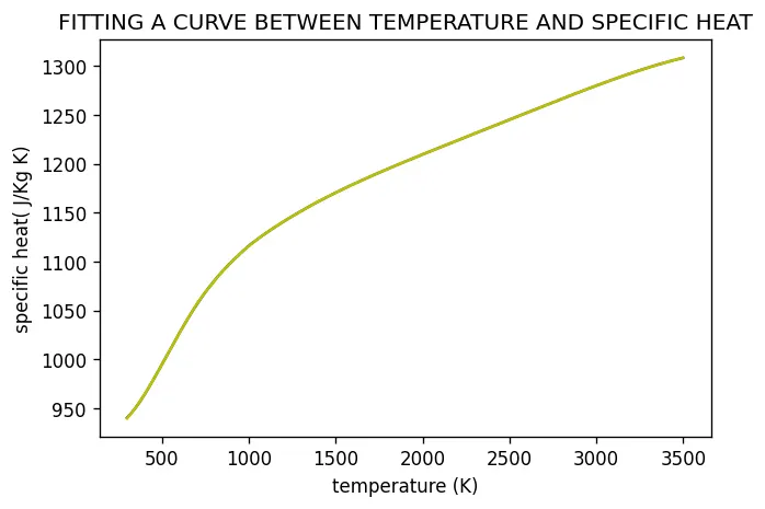
Figure 5:Temperature splitted analysis
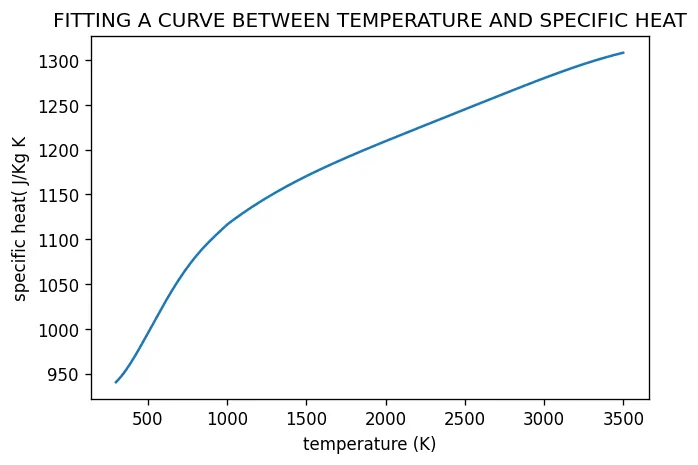
Figure 6:Experimental curve
Both the curves seems to overlap.And thus the curve looks perfect with minimum errors.Thus the goodness of fit is perfect here with minimum errors.