Breaking ice with air cushion vehicle-Find minimum pressure with Newton Raphson method

AIM

write a python script to solve for the minimum value of pressure using the newton raphson method.

OBJECTIVE AND GOVERNING EQUATION

With the given formula as below, solve the following problem.

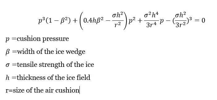
Take β = 0.5, r = 40 feet and σ = 150 pounds per square inch (psi).

1. Use the newton raphson method to find out the value of pressure for h = 0.6 ft.

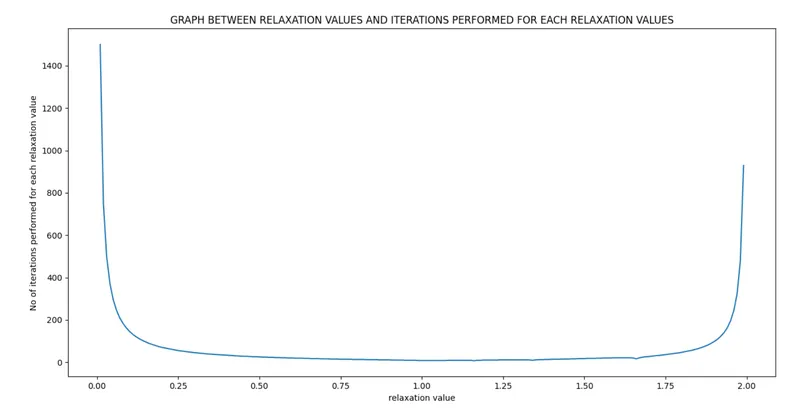
2. Find the optimal relaxation factor for this problem with the help of a suitable plot.

3. Tabulate the results of p for h = [0.6,1.2,1.8,2.4,3,3.6,4.2] assuming a suitable relaxation factor. This must be done in python.

STUDY OBJECTIVE

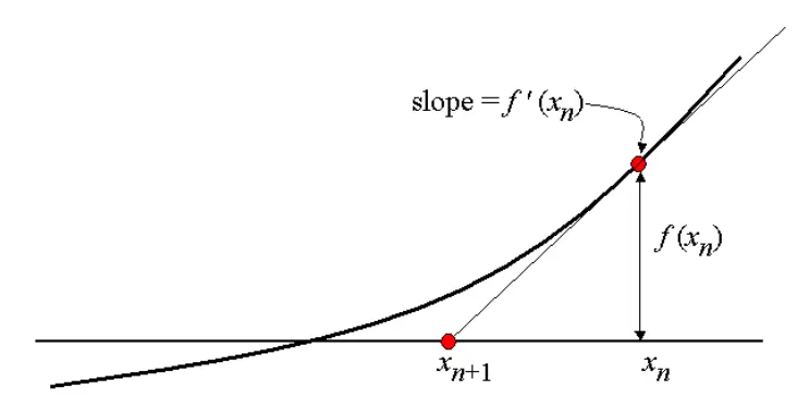
Suppose you need to find the root of a continuous, differentiable function f(x)f(x), and you know the root you are looking for is near the point x=x0​. Then Newton's method tells us that a better approximation for the root is

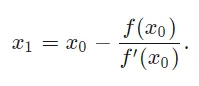
This process may be repeated as many times as necessary to get the desired accuracy. In general, for any x-value x_n​, the next value is given by

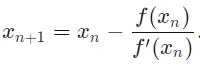
Note: the term "near" is used loosely because it does not need a precise definition in this context. However, x_0x0​ should be closer to the root you need than to any other root (if the function has multiple roots).

Here is a picture to demonstrate what Newton's method actually does:

PROGRAM CODE WITH DETAILED EXPLANATION

Program code for:
Question 1: Use the newton raphson method to find out the value of pressure for h = 0.6 ft.
&
Question 3: Tabulate the results of p for h = [0.6,1.2,1.8,2.4,3,3.6,4.2] assuming a suitable relaxation factor. This must be done in python.

#PROGRAM FOR FINDING CUSHION PRESSURE FOR HEIGHTS MENTIONED USING NEWTON RAPHSON METHOD
#CREATED BY LAKSHMI RAJAN P
#IDLE used : PYCHARM

#Importing the necessary modules for carrying out the program
import math
import matplotlib.pyplot as plt

#Defining the function f(x) as per the equation of cushion pressure as
# p^3(1-b^2)+(0.4*h*b^2-si*h^2/r^2)*p^2+(si^2*h^4*p/3*r^4)-(si*h^2/3*r^2)^3=0
#Entire equation is split to different terms
def f_x(p,b,r,si,h):
    term1=pow(p,3)*(1-pow(b,2))
    term2=pow(p,2)*0.4*h*pow(b,2)
    term3=si*pow(h,2)*pow(p,2)/pow(r,2)
    term4=(p*pow(si,2) * pow(h,4))/(3* pow(r,4))
    term5 = (si*pow(h,2))/(3*pow(r,2))
    term5=pow(term5,3)
    fx=term1+term2-term3+term4-term5
    return fx
#Now the derivation of the function above is found and is divided to different terms
def df_x(p,b,r,si,h):
    term6=3*pow(p,2)*(1-pow(b,2))
    term7=0.8*h*pow(b,2)*pow(p,1)
    term8=2*si*pow(p,1)*pow(h,2)/(pow(r,2))
    term_9=(pow(si,2))*(pow(h,4))/(3*pow(r,4))
    dfx=term6+term7-term8+term_9
    return dfx

#height gives the thickness of the ice field in feet(ft)
height = [0.6, 1.2, 1.8, 2.4, 3, 3.6, 4.2]

#b is the width of the ice wedge
b = 0.5

#r is the size of the air cushion
r = 40
#  tensile strength of the ice is represented as si,given as 150 pounds per sq inch which is converted to feet
# 150*144 pounds per sq feet
si = 21600

# alpha denotes the optimum relaxation value obtained by plotting a graph between relaxation values and its corresponding
# number of iterations

alpha = 1.16
#tolerance is denoted as tol
tol = 1e-4
#Initial assumed value for pressure is denoted as p_guess
p_guess=10
pressure=[]
iteration=[]
iter=0
for i in height:
    p_new=p_guess-(alpha*((f_x(p_guess,b,r,si,i))/(df_x(p_guess,b,r,si,i))))
    pressure.append(p_new)
    iter=iter+1
    iteration.append(iter)
    if(abs(p_new-p_guess)<tol): break="" print('for="" iteration="" no="" ',iter,'the="" pressure="" is="" '="" ,="" p_new="" ,'at="" ',="" i,'ft')="" p_guess="p_new" print("n")="" print('the="" at="" 0.6="" ',round(pressure[0],3))="" #plotting="" the="" graph="" with="" results="" obtained="" plt.plot(height,pressure,"-o")="" plt.xlabel("height="" (in="" feet)")="" plt.ylabel("pressure")="" plt.title("graph="" showing="" relationship="" between="" and="" height")="" plt.show()="" <="" code=""></tol):>

PROCEDURE

1)After thoroughly understanding the concepts on how to find roots of an equation using Newton Raphson method,the given equation is analysed.

2)Now two functions are defined to get the values of f(x) and derivativative of f(x).

3)Now the constant values and variable values are defined.

4)Now for a given set of heights,the pressures are found for each height .

5) for this initial pressure value is assumed and an optimum relaxation value is also assumed.

6)The function is called and the program is run.The result is assigned to some null arrays defined.The loop is run until the condition is violated as specified in the loop.And a plot is drawn between pressure and height.

OUTPUT

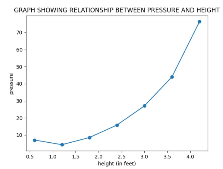
For iteration no  1 the pressure is  7.080528931010599 at height  0.6 ft
For iteration no  2 the pressure is  4.331678527947594 at height  1.2 ft
For iteration no  3 the pressure is  8.52319611439081 at height  1.8 ft
For iteration no  4 the pressure is  15.83104630495902 at height  2.4 ft
For iteration no  5 the pressure is  27.048756744419627 at height  3 ft
For iteration no  6 the pressure is  44.06164996671426 at height  3.6 ft
For iteration no  7 the pressure is  76.33148992683054 at height  4.2 ft


The pressure at height 0.6 is  7.081

The above output is printed on the screen after running the program.The values of pressures for each height is obtained.

The graph obtained between height and pressures are as follows.

Program code with detailed explanation for :

Question 2:

#PROGRAM FOR FINDING THE OPTIMUM RELAXATION VALUE
#CREATED BY LAKSHMI RAJAN P
#IDLE used : PYCHARM

#Importing the necessary modules for carrying out the program
import math
import matplotlib.pyplot as plt
import numpy as np


#Defining the function f(x) as per the equation of cushion pressure as
# p^3(1-b^2)+(0.4*h*b^2-si*h^2/r^2)*p^2+(si^2*h^4*p/3*r^4)-(si*h^2/3*r^2)^3=0
#Entire equation is split to different terms
def f_x(p,b,r,si,h):
    term1=pow(p,3)*(1-pow(b,2))
    term2=pow(p,2)*0.4*h*pow(b,2)
    term3=si*pow(h,2)*pow(p,2)/pow(r,2)
    term4=(p*pow(si,2) * pow(h,4))/(3* pow(r,4))
    term5 = (si*pow(h,2))/(3*pow(r,2))
    term5=pow(term5,3)
    fx=term1+term2-term3+term4-term5
    return fx
#Now the derivation of the function above is found and is divided to different terms
def df_x(p,b,r,si,h):
    term6=3*pow(p,2)*(1-pow(b,2))
    term7=0.8*h*pow(b,2)*pow(p,1)
    term8=2*si*pow(p,1)*pow(h,2)/(pow(r,2))
    term_9=(pow(si,2))*(pow(h,4))/(3*pow(r,4))
    dfx=term6+term7-term8+term_9
    return dfx

#h gives the thickness of the ice field in feet(ft)
h=0.6

#b is the width of the ice wedge
b = 0.5

#r is the size of the air cushion
r = 40

#  tensile strength of the ice is represented as si,given as 150 pounds per sq inch which is converted to feet
# 150*144 pounds per sq feet
si = 21600

#tolerance is denoted as tol
tol = 1e-4

pressure=[]
iteration=[]
a1=[]

#An empty array is set to store the relaxation values in the range 0.01 to 2
for i in range(1,200):
    i=i*0.01
    a1.append(i)
    p_guess = 10
    iter = 1
    #The condition to do the iterations
    while((abs(f_x(p_guess,b,r,si,h)))>tol):
        p_guess=p_guess-(i*((f_x(p_guess,b,r,si,h))/(df_x(p_guess,b,r,si,h))))

        iter=iter+1
    iteration.append(iter)
    pressure.append(p_guess)


#The results are printed
print("The relaxation values are :")
print(a1,end="")
print("n")
print("No of iterations performed for each relaxation value is as follows:  ")
print(iteration)
print('n')
minimum_iteration=min(iteration);
print("The minimum number of iterations coming in the loop is ", minimum_iteration)
optimum_alpha=a1[iteration.index(minimum_iteration)]
print("n")
print("The optimum value of relaxation value for minimum number of iterations is :",optimum_alpha)

#Plotting the results and gettting the graph between relaxation values and the number of iterations
plt.plot(a1,iteration)
plt.title("GRAPH BETWEEN RELAXATION VALUES AND ITERATIONS PERFORMED FOR EACH RELAXATION VALUES")
plt.xlabel("relaxation value")
plt.ylabel("No of iterations performed for each relaxation value")
plt.show()

PROCEDURE

1)After thoroughly understanding the concepts on how to find roots of an equation using Newton Raphson method,the given equation is analysed.

2)Now two functions are defined to get the values of f(x) and derivativative of f(x).

3)Now the constant values and variable values are defined.

4)Now for a given set of relaxation vaues,the pressures are found for given height and the number of iterations required for each is found out.

5) for this initial pressure value is assumed and height is assumed.

6)The function is called and the program is run.The result is assigned to some null arrays defined.The loop is run until the condition is violated as specified in the loop.And a plot is drawn between relaxation values and the number of iterations required to perform the function for each alpha value.

7)Also the optimum relaxation value is found by looking the minimum number of iterations obtained and the correspond relaxation value which takes minimum iteration sto perform the function is considered as the optimum one.

8)The results are printed and the graph is plotted.

OUTPUT

The relaxation values are :
[0.01, 0.02, 0.03, 0.04, 0.05, 0.06, 0.07, 0.08, 0.09, 0.1, 0.11, 0.12, 0.13, 0.14, 0.15, 0.16, 0.17, 0.18, 0.19, 0.2, 0.21, 0.22, 0.23, 0.24, 0.25, 0.26, 0.27, 0.28, 0.29, 0.3, 0.31, 0.32, 0.33, 0.34, 0.35000000000000003, 0.36, 0.37, 0.38, 0.39, 0.4, 0.41000000000000003, 0.42, 0.43, 0.44, 0.45, 0.46, 0.47000000000000003, 0.48, 0.49, 0.5, 0.51, 0.52, 0.53, 0.54, 0.55, 0.56, 0.5700000000000001, 0.58, 0.59, 0.6, 0.61, 0.62, 0.63, 0.64, 0.65, 0.66, 0.67, 0.68, 0.6900000000000001, 0.7000000000000001, 0.71, 0.72, 0.73, 0.74, 0.75, 0.76, 0.77, 0.78, 0.79, 0.8, 0.81, 0.8200000000000001, 0.8300000000000001, 0.84, 0.85, 0.86, 0.87, 0.88, 0.89, 0.9, 0.91, 0.92, 0.93, 0.9400000000000001, 0.9500000000000001, 0.96, 0.97, 0.98, 0.99, 1.0, 1.01, 1.02, 1.03, 1.04, 1.05, 1.06, 1.07, 1.08, 1.09, 1.1, 1.11, 1.12, 1.1300000000000001, 1.1400000000000001, 1.1500000000000001, 1.16, 1.17, 1.18, 1.19, 1.2, 1.21, 1.22, 1.23, 1.24, 1.25, 1.26, 1.27, 1.28, 1.29, 1.3, 1.31, 1.32, 1.33, 1.34, 1.35, 1.36, 1.37, 1.3800000000000001, 1.3900000000000001, 1.4000000000000001, 1.41, 1.42, 1.43, 1.44, 1.45, 1.46, 1.47, 1.48, 1.49, 1.5, 1.51, 1.52, 1.53, 1.54, 1.55, 1.56, 1.57, 1.58, 1.59, 1.6, 1.61, 1.62, 1.6300000000000001, 1.6400000000000001, 1.6500000000000001, 1.6600000000000001, 1.67, 1.68, 1.69, 1.7, 1.71, 1.72, 1.73, 1.74, 1.75, 1.76, 1.77, 1.78, 1.79, 1.8, 1.81, 1.82, 1.83, 1.84, 1.85, 1.86, 1.87, 1.8800000000000001, 1.8900000000000001, 1.9000000000000001, 1.9100000000000001, 1.92, 1.93, 1.94, 1.95, 1.96, 1.97, 1.98, 1.99]

No of iterations performed for each relaxation value is as follows:  
[1501, 748, 497, 372, 296, 246, 210, 184, 163, 146, 132, 121, 111, 103, 96, 89, 84, 79, 74, 70, 67, 64, 61, 58, 55, 53, 51, 49, 47, 45, 44, 42, 41, 39, 38, 37, 36, 35, 34, 33, 32, 31, 30, 29, 28, 28, 27, 26, 26, 25, 24, 24, 23, 23, 22, 22, 21, 21, 20, 20, 19, 19, 19, 18, 18, 17, 17, 17, 16, 16, 16, 15, 15, 15, 14, 14, 14, 14, 13, 13, 13, 13, 12, 12, 12, 12, 11, 11, 11, 11, 10, 10, 10, 10, 9, 9, 9, 9, 8, 8, 8, 8, 8, 8, 8, 8, 8, 9, 9, 9, 9, 9, 9, 9, 9, 7, 9, 9, 10, 10, 10, 10, 10, 11, 11, 11, 11, 11, 11, 11, 11, 11, 11, 9, 11, 12, 12, 13, 13, 14, 14, 14, 15, 15, 15, 16, 16, 17, 17, 17, 18, 18, 18, 19, 19, 20, 20, 20, 21, 21, 21, 21, 21, 21, 20, 16, 21, 24, 26, 27, 29, 31, 32, 34, 36, 38, 40, 42, 44, 47, 50, 53, 56, 60, 64, 69, 75, 81, 89, 98, 109, 123, 140, 163, 196, 244, 322, 478, 929]


The minimum number of iterations coming in the loop is  7


The optimum value of relaxation value for minimum number of iterations is : 1.16

The above output is got while running the program,where the optimum relaxation value is found out and a graph is plotted as below.