Curve fitting using PYTHON

Objective: -

The main objective is to perform a curve fit for the given set of data and explain the python codes used in developing the program with the explanation of the theoretical question asked above

Principle: -

Curve fitting refers to finding an appropriate mathematical model that expresses the relationship between a dependent variable Y and a single independent variable X. It is the process of constructing a curve or mathematical function, that has the best fit to a series of data points possibly subject to constraints. Curve fitting can involve either interpolation where an exact fit to the data is required, in which a "smooth" function is constructed that approximately fits the data

If an appropriate function f can be found for an experiment we can use the equation to determine physical parameters related to the experiment, and we can use this new model to predict new things about the world. Galileo used this method to calculate the trajectory of cannonballs by rolling them down inclined ramps.

In experimental physics, we constrain these models by designing an experiment with two quantities. The first quantity, that we can control, is the independent variable. The second quantity, that we can measure, is the dependent variable. The relationship between these two quantities can then be used to determine some physical parameters.

A simple example of measuring the path of the moving object. We could guess that the model is moving at a constant speed and design an experiment to find that speed using the model:

s=ut">s=ut

s=ut">Scipy provides a function that can fit model functions to the data

Scipy provides a number of functions that, given a suitable model function, can return the best estimate of the unknown parameters in the model.

Consider the experiment where the time of flight of an object moving at constant speed is measured. If the experiment is correctly setup. The unknown variable we are trying to determine is the speed uu. The remaining variables are time t and height s. We can design two different experiments, one where we control time (measuring at a fixed interval) and measure distance or one where we control distance and measure time.

Solution Procedure: -

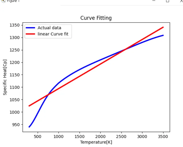
• Linear: y=a+bx">y=a+bxy=a+bx

This common model is usually fit using standard linear regression techniques. We include it here to allow for
various special forms made by transforming X and Y

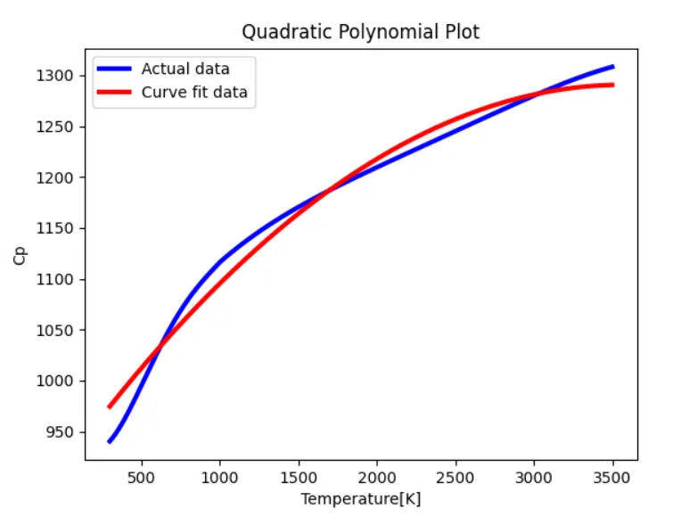
• Quadratic: y=a+bx+cx2">y=a+bx+cx2y=a+bx+cx2

The quadratic or second-order polynomial model results in the familiar parabola.

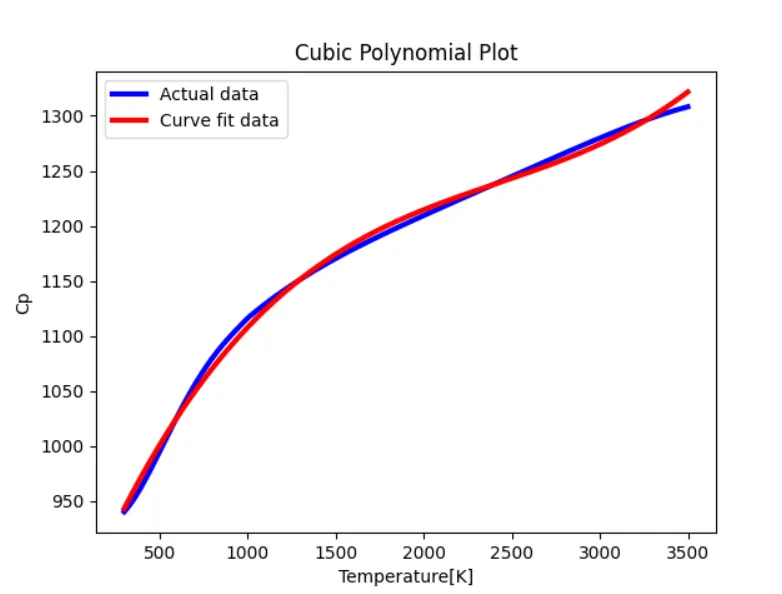
• Cubic: y=a+bx+cx2+dx3">y=a+bx+cx2+dx3y=a+bx+cx2+dx3

This is the cubic or third-order polynomial

Curve fit algorithms determine the best-fit parameters by minimizing a chosen merit function. In order to optimize the merit function, it is necessary to select a set of initial parameter estimates and then iteratively refine the merit parameters until the merit function does not change significantly between iterations.

Error(i) =|y(i) - value of function y = f(x) at x=x(i)| = |y(i) - value of f(x) at x(i)|

Fitting Techniques: -

1. Fourier to fit data similar to the waveform
2. Linear fitting doing the first-order fit directly for the selected data set
3. The polynomial fit - general polynomial of any particular order to fit the dataset
4. Interpolant method - create a curve/surface passing all the data point

The parameter used to measure the fitness of the curve: -

• SSE(Sum of the square term) - This statistic measures the total deviation of the response values from the fit to the response values. It is also called the summed square of residuals and is usually labeled as SSE

SSE=∑i=1nErr(i)2">SSE=∑ni=1Err(i)2SSE=∑i=1nErr(i)2

A value closer to 0 indicates that the model has a smaller random error component and that the fit will be more useful for prediction.

• R-Square

  This statistic measures how successful the fit is in explaining the variation of the data. Put another way, R-square is the square of the correlation between the response values and the predicted response values. It is also called the square of the multiple correlation coefficient and the coefficient of multiple determination.

R-square=SSR/SST

• Degrees of Freedom Adjusted R-Square

  This statistic uses the R-square statistic defined above and adjusts it based on the residual degrees of freedom. The residual degrees of freedom is defined as the number of response values n minus the number of fitted coefficients m estimated from the response values.

  v = n – m

  v indicates the number of independent pieces of information involving the n data points that are required to calculate the sum of squares. Note that if parameters are bounded and one or more of the estimates are at their bounds, then those estimates are regarded as fixed. The degrees of freedom are increased by the number of such parameters.

  The adjusted R-square statistic is generally the best indicator of the fit quality when you compare two models that are nested — that is, a series of models each of which adds additional coefficients to the previous model.

  adjusted R-square=1−SSE(n−1)SST(v)

  The adjusted R-square statistic can take on any value less than or equal to 1, with a value closer to 1 indicating a better fit. Negative values can occur when the model contains terms that do not help to predict the response.

  Root Mean Squared Error

  This statistic is also known as the fit standard error and the standard error of the regression. It is an estimate of the standard deviation of the random component in the data and is defined as

  RMSE=s= M2SE">2√MSEM2SE

Based on the research I have done:-

How to make a curve fit perfectly?

The curve fit is known to be a perfect fit when the predicted curve points and the actual curve points meet at all the points and the value for the R square is 1.Increasing the number of polynomials thus, increase the probability of a more fitter curve. Perfect can always be the best fit but the best fit can not be a perfect fit, we can get a perfect fit with a 3-degree polynomial but it is not the best fit as for the best fit we can increase the degree of the polynomial

How to get the best fit?

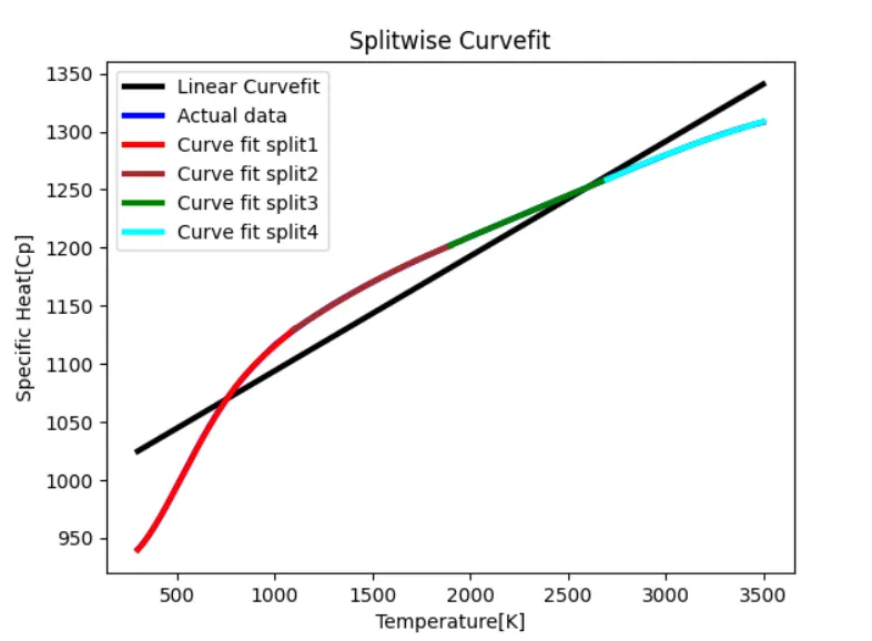
We can get the best fit by increasing the degree of the polynomial and can also use RMSE and also we can use splitwise method to split the data into folds and perform a curve fit to get the best fit

What could be done to improve the cubic fit?

We can improve the cubic fit by increasing the degree of a polynomial or by using the splitwise method to get an improved cubic fit

What do popt and pcov mean?

• popt - is a one-dimensional array of the best estimates for the parameter values, each entry matches the order in the function definition.it gives an array for the optimal values of the parameters so that square residuals of the data is minimized
• pcov - is the covariance matrix showing the uncertainty and interdependence of each parameter in popt. We take the diagonal elements as pvar for the variance of each parameter in popt. It is a 2D array with the estimated covariance of the parameters in popt. The pcov variable contains the covariance matrix, which indicates the uncertainties and correlations between parameters. This is most useful when the data has uncertainties

What do np.array(temperature) mean?

It generates an array and stores the different values of the temperature and passes the generated value to the NumPy for numerical calculation in python.

What does the * in *popt mean?

It refers to the value in the array popt

What needs to be done in order to make the curve fit perfectly?

To make the curve fit perfectly fit on the actual curve by using the high-level order polynomial or splitwise method can be used to fit it by dividing the data into different folds and plot on the curve as per the requirement

CODE for the Linear Curvefit:-

#linearfit curve code
import numpy as np
import matplotlib.pyplot as plt
from scipy.optimize import curve_fit

#Curve fit function


def func1(r,x,y):
	return x*r+y


#Reading thermodynamic data file
def read_file():
	temp =[]
	cp=[]

	for line in open('data','r'):
		values = line.split(',')
		temp.append(float(values[0]))
		cp.append(float(values[1]))

	return [temp, cp]



#Main code for curve fit by splitting curve in different parts or four folds 
temp ,cp =read_file()

#linear fit
popt , pcov = curve_fit(func1,temp,cp)
fit_cp = func1(np.array(temp),*popt)
plt.plot(temp,cp,color ='blue',linewidth =3)

plt.plot(temp,fit_cp,color ='red',linewidth =3)

plt.legend(['Actual data','Curve fit split1','Curve fit split2','Curve fit split3','Curve fit split4'])
plt.xlabel('Temperature[K]')
plt.ylabel('Specific Heat[Cp]')
plt.show()

Explanation of the above code: -

import numpy as np - importing the numpy library
import matplotlib.pyplot as plt - importing the matplot library for the plot
from scipy.optimize import curve_fit - importing the scipy optimize module for the curve fit plotting

#Curve fit function - comment to make a program a program user friendly

def func1(r,x,y): - defining the function to perform a linear fit curvefit
return x*r+y - return statement is used to return a value when called

#Reading thermodynamic data file
def read_file(): - defining a function to read a given set of data`
temp =[] - a temperature array is assigned to store the temperature
cp=[] - a specific heat array is generated to store the value

for line in open('data','r'): - for loop to open a file naming data
values = line.split(',') - values store the assign value split by (,)
temp.append(float(values[0])) - in temperature array the float values of the diff temperature above extracted is stored or appended
cp.append(float(values[1])) - in cp array the float values of the diff cp above extracted is stored or appended

return [temp, cp] - return statement to return the values

#Main code for curve fit by splitting curve in different parts or four folds
temp ,cp =read_file() - as the read_file function returns two values so temp and cp is assigned to store their values

#linear fit - comments
popt , pcov = curve_fit(func1,temp,cp) - is a one-dimensional array of the best estimates for the parameter values, each entry matches the order in the function definition , The pcov variable contains the covariance matrix
fit_cp = func1(np.array(temp),*popt) - fit_cp store the value of popt It generates an array and stores the different values of the temperature and passes the generated value to the NumPy for numerical calculation in python and refers to value in the array popt
plt.plot(temp,cp,color ='blue',linewidth =3) - ploting of the original curve in blue color

plt.plot(temp,fit_cp,color ='red',linewidth =3) - plotting the linear value of the plot in red color

plt.legend(['Actual data','Curve fit ']) - legend is plotted with actual curve and curve fit

plt.xlabel('Temperature[K]')- labeling the x axis
plt.ylabel('Specific Heat[Cp]') - labelling the y axis
plt.show() - to show the plot in the output window

________________________________________________________________________________________________________

Output for Linear Curvefit: -

CODE for the Quadratic Curvefit:-

import numpy as np
import matplotlib.pyplot as plt
from scipy.optimize import curve_fit

#Curve fit function

def func(r,x,y,z):
	return x*pow(r,2)+y*r +z


#Reading thermodynamic data file

def read_file():
	temp =[]
	cp=[]

	for line in open('data','r'):
		values = line.split(',')
		temp.append(float(values[0]))
		cp.append(float(values[1]))

	return [temp, cp]

#Main code for curve fit
temp ,cp =read_file()
popt , pcov = curve_fit(func,temp,cp)
fit_cp = func(np.array(temp),*popt)


plt.plot(temp,cp,color ='blue',linewidth =3)
plt.plot(temp,fit_cp,color ='red',linewidth =3)
plt.legend(['Actual data','Curve fit data'])
plt.title('Quadratic Polynomial Plot')
plt.xlabel('Temperature[K]')
plt.ylabel('Cp')
plt.show()

Explanation of the above code: -

import numpy as np - importing the numpy library
import matplotlib.pyplot as plt - importing the matplot library for the plot
from scipy.optimize import curve_fit - importing the scipy optimize module for the curve fit plotting

#Curve fit function - comment to make a program a program user friendly

def func1(r,x,y,z): - defining the function to perform a quadratic fit curvefit
return x*pow(r,2)+y*r +z- return statement is used to return a value when called

#Reading thermodynamic data file
def read_file(): - defining a function to read a given set of data`
temp =[] - a temperature array is assigned to store the temperature
cp=[] - a specific heat array is generated to store the value

for line in open('data','r'): - for loop to open a file naming data
values = line.split(',') - values store the assign value split by (,)
temp.append(float(values[0])) - in temperature array the float values of the diff temperature above extracted is stored or appended
cp.append(float(values[1])) - in cp array the float values of the diff cp above extracted is stored or appended

return [temp, cp] - return statement to return the values

#Main code for curve fit by splitting curve in different parts or four folds
temp ,cp =read_file() - as the read_file function returns two values so temp and cp is assigned to store their values

#quadraticfit - comments
popt , pcov = curve_fit(func1,temp,cp) - is a one-dimensional array of the best estimates for the parameter values, each entry matches the order in the function definition , The pcov variable contains the covariance matrix
fit_cp = func1(np.array(temp),*popt) - fit_cp store the value of popt It generates an array and stores the different values of the temperature and passes the generated value to the NumPy for numerical calculation in python and refers to value in the array popt
plt.plot(temp,cp,color ='blue',linewidth =3) - ploting of the original curve in blue color

plt.plot(temp,fit_cp,color ='red',linewidth =3) - plotting the quadratic value of the plot in red color

plt.legend(['Actual data','Curve fit ']) - legend is plotted with actual curve and curve fit

plt.xlabel('Temperature[K]')- labeling the x axis
plt.ylabel('Specific Heat[Cp]') - labelling the y axis
plt.show() - to show the plot in the output window

Output: -

CODE for the Cubic Curvefit:-

import numpy as np
import matplotlib.pyplot as plt
from scipy.optimize import curve_fit

#Curve fit function


def func(r,x,y,z,p):
	return x*pow(r,3)+y*pow(r,2) +z*r+p

#Reading thermodynamic data file

def read_file():
	temp =[]
	cp=[]

	for line in open('data','r'):
		values = line.split(',')
		temp.append(float(values[0]))
		cp.append(float(values[1]))

	return [temp, cp]

#Main code for curve fit
temp ,cp =read_file()
popt , pcov = curve_fit(func,temp,cp)
fit_cp = func(np.array(temp),*popt)


plt.plot(temp,cp,color ='blue',linewidth =3)
plt.plot(temp,fit_cp,color ='red',linewidth =3)
plt.legend(['Actual data','Curve fit data'])
plt.title('Cubic Polynomial Plot')
plt.xlabel('Temperature[K]')
plt.ylabel('Cp')
plt.show()

Explanation of the above code: -

import numpy as np - importing the numpy library
import matplotlib.pyplot as plt - importing the matplot library for the plot
from scipy.optimize import curve_fit - importing the scipy optimize module for the curve fit plotting

#Curve fit function - comment to make a program a program user friendly

def func1(r,x,y,z,p): - defining the function to perform a quadratic fit curvefit
return x*pow(r,3)+y*pow(r,2) +z*r+p- return statement is used to return a value when called

#Reading thermodynamic data file
def read_file(): - defining a function to read a given set of data`
temp =[] - a temperature array is assigned to store the temperature
cp=[] - a specific heat array is generated to store the value

for line in open('data','r'): - for loop to open a file naming data
values = line.split(',') - values store the assign value split by (,)
temp.append(float(values[0])) - in temperature array the float values of the diff temperature above extracted is stored or appended
cp.append(float(values[1])) - in cp array the float values of the diff cp above extracted is stored or appended

return [temp, cp] - return statement to return the values

#Main code for curve fit by splitting curve in different parts or four folds
temp ,cp =read_file() - as the read_file function returns two values so temp and cp is assigned to store their values

#cubicfit - comments
popt , pcov = curve_fit(func1,temp,cp) - is a one-dimensional array of the best estimates for the parameter values, each entry matches the order in the function definition , The pcov variable contains the covariance matrix
fit_cp = func1(np.array(temp),*popt) - fit_cp store the value of popt It generates an array and stores the different values of the temperature and passes the generated value to the NumPy for numerical calculation in python and refers to value in the array popt
plt.plot(temp,cp,color ='blue',linewidth =3) - ploting of the original curve in blue color

plt.plot(temp,fit_cp,color ='red',linewidth =3) - plotting the Cubic polynomial value of the plot in red color

plt.legend(['Actual data','Curve fit ']) - legend is plotted with actual curve and curve fit

plt.xlabel('Temperature[K]')- labeling the x axis
plt.ylabel('Specific Heat[Cp]') - labelling the y axis
plt.show() - to show the plot in the output window

Output for the Cubic Plot: -

________________________________________________________________________________________________________

CODE for the Split Curvefit in four folds:-

import numpy as np
import matplotlib.pyplot as plt
from scipy.optimize import curve_fit

#Curve fit function
def func2(r,x,y,z,p,q):
	return x*pow(r,4)+y*pow(r,3) +z*pow(r,2)+p*r+q

def func(r,x,y,z,p):
	return x*pow(r,3)+y*pow(r,2) +z*r+p

def func1(r,x,y):
	return x*r+y

def func3(r,x,y,z):
	return x*pow(r,2)+y*r +z

#Reading thermodynamic data file
def read_file():
	temp =[]
	cp=[]

	for line in open('data','r'):
		values = line.split(',')
		temp.append(float(values[0]))
		cp.append(float(values[1]))

	return [temp, cp]



#Main code for curve fit by splitting curve in different parts or four folds 
temp ,cp =read_file()

#linear fit
popt , pcov = curve_fit(func1,temp,cp)
fit_cp = func1(np.array(temp),*popt)
plt.plot(temp,fit_cp,color ='black',linewidth =3)

#main curve or actual
popt , pcov = curve_fit(func,temp,cp)
fit_cp = func(np.array(temp),*popt)

#for temp1 and cp1
temp1 = temp[0:800]
cp1 = cp[0:800]
popt1, pcov1 = curve_fit(func2,temp1,cp1)
fit_cp1 = func2(np.array(temp1),*popt1)

#for temp2 and cp2
temp2 = temp[800:1600]
cp2 = cp[800:1600]
popt2, pcov2 = curve_fit(func3,temp2,cp2)
fit_cp2 = func3(np.array(temp2),*popt2)

#for temp3 and cp3
temp3 = temp[1600:2400]
cp3 = cp[1600:2400]
popt3, pcov3 = curve_fit(func2,temp3,cp3)
fit_cp3 = func2(np.array(temp3),*popt3)

#for temp4 and cp4
temp4 = temp[2400:3400]
cp4 = cp[2400:3200]
popt4, pcov4 = curve_fit(func3,temp4,cp4)
fit_cp4 = func3(np.array(temp4),*popt4)


plt.plot(temp,cp,color ='blue',linewidth =3)

plt.plot(temp1,fit_cp1,color ='red',linewidth =3)
plt.plot(temp2,fit_cp2,color ='brown',linewidth =3)
plt.plot(temp3,fit_cp3,color ='green',linewidth =3)
plt.plot(temp4,fit_cp4,color ='cyan',linewidth =3)

#to calculate the goodness of a fit


plt.title('Splitwise Curvefit')
plt.legend(['Linear Curvefit','Actual data','Curve fit split1','Curve fit split2','Curve fit split3','Curve fit split4'])
plt.xlabel('Temperature[K]')
plt.ylabel('Specific Heat[Cp]')
plt.show()

def r_sq(temp,cp,fit_cp):
	for i in range(0,len(temp)):
		Mean = np.mean(cp)
		ssr = np.sum(pow((fit_cp[i]-Mean),2))
		sse = np.sum(pow((cp[i]-fit_cp[i]),2))
		sst = ssr+sse
		r_2 = ssr/sst
	return r_2

goodness_fit = r_sq(temp,cp,fit_cp)
k1 = r_sq(temp1,cp1,fit_cp1)
k2 = r_sq(temp2,cp2,fit_cp2)
k3 = r_sq(temp3,cp3,fit_cp3)
k4 = r_sq(temp4,cp4,fit_cp4)

#Best fit
Bf = (k1+k2+k3+k4)/4
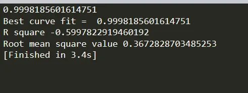
print(Bf)

if(Bf> 0.9):
	print('Best curve fit = ',Bf)

#R square adjustment 
#let p =8
p = 8
#number of data points
n =len(pcov) 
r_adjust = 1- (abs(1-pow(Bf,2)*(n-1)/(n-p-1)))
print('R square =',r_adjust)

#Root mean square method to identify goodness of the fit

for j in range(0,len(pcov)):
	sse  =np.sum(pcov[j])

rmse = np.math.sqrt(sse/n)
print('Root mean square value =',rmse)

Explanation of the above code: -

import numpy as np - importing the numpy library
import matplotlib.pyplot as plt - importing the matplot library for the plot
from scipy.optimize import curve_fit - importing the scipy optimize module for the curve fit plotting

#Curve fit function - comments

def func(r,x,y,z,p): - defining the function to perform a cubic fit curve fit
return x*pow(r,3)+y*pow(r,2) +z*r+p

def func1(r,x,y):- defining the function to perform a linear fit curve fit
return x*r+y

def func2(r,x,y,z,p,q):- defining the function to perform a high order polynomial fit curve fit
return x*pow(r,4)+y*pow(r,3) +z*pow(r,2)+p*r+q

def func3(r,x,y,z): - defining the function to perform a qudratic fit curve fit
return x*pow(r,2)+y*r +z

#Reading thermodynamic data file
def read_file(): - defining a function to read a given set of data`
temp =[] - a temperature array is assigned to store the temperature
cp=[] - a specific heat array is generated to store the value

for line in open('data','r'): - for loop to open a file naming data
values = line.split(',') - values store the assign value split by (,)
temp.append(float(values[0])) - in temperature array the float values of the diff temperature above extracted is stored or appended
cp.append(float(values[1])) - in cp array the float values of the diff cp above extracted is stored or appended

return [temp, cp] - return statement to return the values

#Main code for curve fit by splitting curve in different parts or four folds
temp ,cp =read_file() - as the read_file function returns two values so temp and cp is assigned to store their values

#linear fit
popt , pcov = curve_fit(func1,temp,cp)
fit_cp = func1(np.array(temp),*popt)
plt.plot(temp,fit_cp,color ='black',linewidth =3)

#main curve or actual
popt , pcov = curve_fit(func,temp,cp)
fit_cp = func(np.array(temp),*popt)

#for temp1 and cp1
temp1 = temp[0:800] - splitting the temperature range 0 to 800 k
cp1 = cp[0:800] - splitting the temperature
popt1, pcov1 = curve_fit(func2,temp1,cp1) - is a one-dimensional array of the best estimates for the parameter values, each entry matches the order in the function definition , The pcov variable contains the covariance matrix
fit_cp1 = func2(np.array(temp1),*popt1) - fit_cp store the value of popt It generates an array and stores the different values of the temperature and passes the generated value to the NumPy for numerical calculation in python and refers to value in the array popt

#for temp2 and cp2
temp2 = temp[800:1600]- splitting the temperature range 800 to 1600 k
cp2 = cp[800:1600] - cp2 saves the cp range from 800 and 1600
popt2, pcov2 = curve_fit(func3,temp2,cp2)
fit_cp2 = func3(np.array(temp2),*popt2)

#for temp3 and cp3
temp3 = temp[1600:2400]- splitting the temperature range 1600 to 2400 k
cp3 = cp[1600:2400]
popt3, pcov3 = curve_fit(func2,temp3,cp3)
fit_cp3 = func2(np.array(temp3),*popt3)

#for temp4 and cp4
temp4 = temp[2400:3400]
cp4 = cp[2400:3200]
popt4, pcov4 = curve_fit(func3,temp4,cp4)
fit_cp4 = func3(np.array(temp4),*popt4)

plt.plot(temp,cp,color ='blue',linewidth =3) -plotting the actual curve

plt.plot(temp1,fit_cp1,color ='red',linewidth =3) -plotting of the high order polynomialcurvefit for the given range of temp and cp
plt.plot(temp2,fit_cp2,color ='brown',linewidth =3)- plotting of the quadratic curvefit for the given range of temp and cp
plt.plot(temp3,fit_cp3,color ='green',linewidth =3)plotting of the curvefit for the given range of temp and cp
plt.plot(temp4,fit_cp4,color ='cyan',linewidth =3) - plotting of the curvefit for the given range of temp and cp

def r_sq(temp,cp,fit_cp): - defining a function r_sq to solve ssr/sst
for i in range(0,len(temp)): - for loop in range 0 to length of temperature
Mean = np.mean(cp) - mean initialize with the np.mean calculation value
ssr = np.sum(pow((fit_cp[i]-Mean),2)) - ssr is solved according to the equation
sse = np.sum(pow((cp[i]-fit_cp[i]),2))- sse is solved according to the equation
sst = ssr+sse - sst is solved according to the equation ssr+sse
r_2 = ssr/sst - is solved according to the equation
return r_2 - value is returned by the function

goodness_fit = r_sq(temp,cp,fit_cp) - store the value returned from the function above
k1 = r_sq(temp1,cp1,fit_cp1) - store the value returned from the function above
k2 = r_sq(temp2,cp2,fit_cp2) - store the value returned from the function above
k3 = r_sq(temp3,cp3,fit_cp3) - store the value returned from the function above
k4 = r_sq(temp4,cp4,fit_cp4) - store the value returned from the function above

#Best fit - comments to make a program user friendly
Bf = (k1+k2+k3+k4)/4 - calculating the best fit
print(Bf) - printing the best fit

if(Bf> 0.9): - checking the bf value using if statement
print('Best curve fit = ',Bf) - print the value of the best fit curve

#R square adjustment
#let p =8
p = 8
#number of data points
n =len(pcov) - to store the length of the pcov intialize above in code
r_adjust = 1- (abs(1-pow(Bf,2)*(n-1)/(n-p-1))) - calculating r adjusted value according to the equation
print('R square =',r_adjust) - printing the value of r square

#Root mean square method to identify goodness of the fit

for j in range(0,len(pcov)): - running a loop till length of pcov
sse =np.sum(pcov[j]) - initializing sse as sum of pcov array value

rmse = np.math.sqrt(sse/n) - rmse to store the sqrt value of sse/n
print('Root mean square value =',rmse) - printing the rmse value

plt.title('Splitwise Curvefit') - title given to the plot
plt.legend(['Actual data','Curve fit split1','Curve fit split2','Curve fit split3','Curve fit split4']) - legend are given to the plot
plt.xlabel('Temperature[K]') - labelling the x axis
plt.ylabel('Specific Heat[Cp]') - labelling the y axis
plt.show() - to show the plot in the output window

Output of the splitwise plot: -

_______________________________________________________________________________________________________

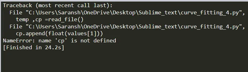
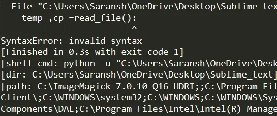
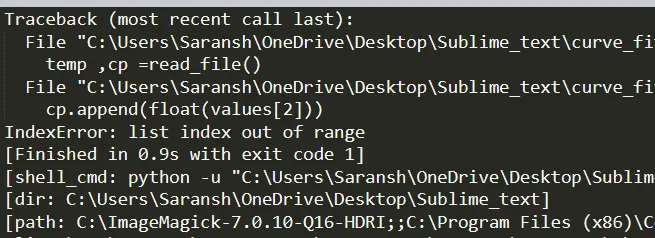
Error faced during programming: -

• variable not found on debugging it was found error was due to wrong variable name

• invalid syntax was found but on debugging (:) it was used in the wrong place

• The output window doesn't show any plot as plt.show() was missing

• There was a index out of bond as the values[2] was wrong

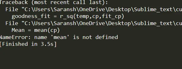
• The mean statement was not valid. on debugging it was found that np.mean was to be used

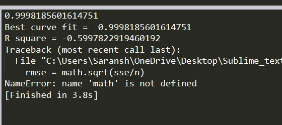
• The math.sqrt was used so syntax index was found on debugging it was found np.math.sqrt was used

References: -

http://phy224.ca/19-curvefit/index.html

https://skill-lync.com/projects/Curve-Fitting-and-criterion-to-choose-best-fit-41860

https://astrofrog.github.io/py4sci/_static/15.%20Fitting%20models%20to%20data.html